Mistakes Data Scientists Make

Introduction

Patterns exist in the mistakes data scientists make - this article lists some of the most common mistakes data scientists make when learning their craft.

An expert is a person who has made all the mistakes that can be made in a very narrow field.

Niels Bohr

I’ve learnt from all these mistakes - I hope you can learn from them too.

Plot the Target

Prediction separates the data scientist from the data analyst. The data analyst analyzes the past - the data scientist predicts the future.

Using features to predict a target is supervised learning. The target can be either a number (regression) or a category (classification).

Understanding the distribution of the target is a must-do for any supervised learning project.

The distribution of the target will inform many decisions a data scientist makes, including:

• what models to consider using
• whether scaling is required
• if the target has outliers that should be removed
• if the target is imbalanced

Regression

In a regression problem, a data scientist wants to know the following about the target:

• the minimum & maximum
• how normally distributed the target it
• if the distribution is multi-modal
• if there are outliers

A histogram will answer all of these - making it an excellent choice for visualizing the target in regression problems.

The code below generates a toy dataset of four distributions and plots a histogram:

import numpy as np
import pandas as pd

data = np.concatenate([
    np.random.normal(5, 1, 10000),
    np.random.normal(-5, 1, 10000),
    np.array([-20, 20] * 1000)
])
ax = pd.DataFrame(data).plot(kind='hist', legend=None, bins=100)

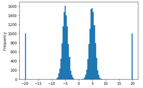
The histogram shows the two normal and two uniform distributions that generated this dataset.

Classification

In a classification problem, a data scientist wants to know the following about the target:

• how many classes there are
• how balanced are the classes

We can answer these questions using a single bar chart:

import pandas as pd

data = ['awake'] * 1000 + ['asleep'] * 500 + ['dreaming'] * 50
ax = pd.Series(data).value_counts().plot(kind='bar')

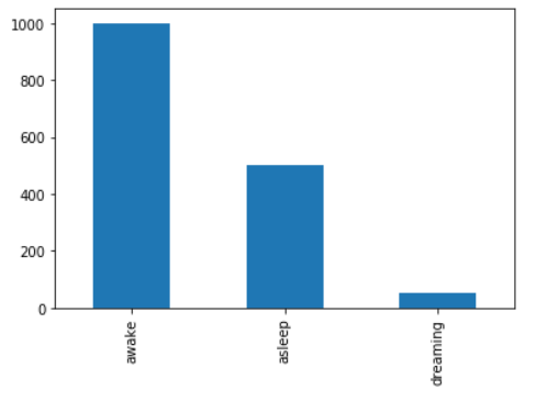
The bar chart shows us we have three classes, and shows our dreaming class is under-represented.

Dimensionality

Dimensionality provides structure for understanding the world. An experienced data scientist learns to see the dimensions of data.

The Value of Low Dimensional Data

In business, lower dimensional representations are more valuable than high dimensional representations. Business decisions are made in low dimensional spaces.

Notice that much of the work of a data scientist is using machine learning to reduce dimensionality:

• using pixels in an satellite image to predict solar power output,
• using wind turbine performance data to estimate the probability of future breakdown,
• using customer data to predict customer lifetime value.

Each of the outputs can be used by a business ways the raw data can’t. Unlike their high dimensional raw data inputs, the lower dimensional outputs can be used to make decisions:

• solar power output can be used to guide energy trader actions,
• a high wind turbine breakdown probability can lead to a maintenance team being sent out,
• a low customer lifetime estimation can lead to less money budgeting for marketing.

The above are examples of the interaction between prediction and control. The better you are able to predict the world, the better you can control it.

This is also a working definition of a data scientist - making predictions that lead to action - actions that change how a business is run.

The Challenges of High Dimensional Data

The difficulty of working in high dimensional spaces is known as the curse of dimensionality.

To understand the curse of dimensionality we need to reason about the space and density of data. We can imagine a dense dataset - a large number of diverse samples within a small space. We can also imagine a sparse dataset - a small number of samples in a large space.

What happens to the density of a dataset as we add dimensions? It becomes less dense, because the data is now more spread out.

However, the decrease of data density with increasing dimensionality is not linear - it’s exponential. The space becomes exponentially harder to understand as we increase dimensions.

Why is the increase exponential? Because this new dimension needs to be understood not only in terms of the each other dimension (which would be linear) but in terms of the combination of every other dimension with every other dimension (which is exponential).

This is the curse of dimensionality - the exponential increase of space as we add dimensions. The code below show this effect:

import itertools

def calc_num_combinations(data):
    return len(list(itertools.permutations(data, len(data))))

def test_calc_num_combinations():
    """To test it works :)"""
    test_data = (((0, ), 1), ((0, 1), 2), ((0, 1, 2), 6))
    for data, length in test_data:
        assert length == calc_num_combinations(data)

test_calc_num_combinations()
print([(length, calc_num_combinations(range(length))) for length in range(11)])
"""
[(0, 1),
 (1, 1),
 (2, 2),
 (3, 6),
 (4, 24),
 (5, 120),
 (6, 720),
 (7, 5040),
 (8, 40320),
 (9, 362880),
 (10, 3628800)]
"""

The larger the size of the space, the more work a machine learning model needs to do to understand it.

This is why adding features with no signal is painful. Not only does the model need to learn it’s noise - it needs to do this by considering how this noise interacts with each combination of every other column.

Applying the Curse of Dimensionality

Getting a theoretical understanding of dimensionality is step one. Next is applying it in the daily practice of data science. Below we will go through a few practical cases where data scientists can not apply the curse of dimensionality to their own workflow.

Too Many Hyperparameters

Data scientists can waste time doing excessive grid searching - expensive in both time and compute. The motivation of complex grid searches come from a good place - the desire for good (or even perfect) hyperparameters.

Yet we now know that adding just one additional search means an exponential increase in models trained - because this new search parameter needs to be tested in combination with every other search parameter.

Another mistake is narrow grid searches - searching over small ranges of hyperparameters. A logarithmic scale will be more informative than a small linear range:

#  this search isn't wide enough
useless_search = sklearn.model_selection.GridSearchCV(
    sklearn.ensemble.RandomForestRegressor(n_estimators=10), param_grid={'n_estimators': [10, 15, 20]
)

#  this search is more informative
useful_search = sklearn.model_selection.GridSearchCV(
    sklearn.ensemble.RandomForestRegressor(n_estimators=10), param_grid={'n_estimators': [10, 100, 1000]
)

• one to compare different models (using the best hyperparameters found so far for each)
• one to compare different hyperparameters for a single model

I’ll start by comparing models in the first pipeline, then doing further tuning on a single model in the second grid search pipeline. Once a model is reasonably tuned, it’s best hyperparameters can be put into the first grid search pipeline.

The fine tuning on a single model is often searches over a single parameter at a time (two maximum). This keeps the runtime short, and also helps to develop intuition about what effect changing hyperparameters will have on model performance.

Too Many Features

A misconception I had as a junior data scientist was that adding features had no cost. Put them all in and let the model figure it out! We can now easily see the naivety of this - more features has as exponential cost.

This misconception came from a fundamental misunderstanding of deep learning.

Seeing the results in computer vision, where deep neural networks do all the work of feature engineering from raw pixels, I thought that the same would be true of using neural networks on other data. I was making two mistakes here:

• not appreciating the useful inductive bias of convolutional neural networks
• not appreciating the curse of dimensionality

We know now there is an exponential cost to adding more features. This also should change how you look at one-hot encoding, which dramatically increases the space that a model needs to understand, with low density data.

Too Many Metrics

In data science projects, performance is judged using metrics such as training or test performance.

In industry, a data scientist will choose metrics that align with the goals of the business. Different metrics have different trade-offs - part of a data scientists job is to select metrics that correlate best with the objectives of the business.

However, it’s common for junior data scientists to report a range of different metrics. For example, on a regression problem they might report three metrics:

• mean absolute error
• mean absolute percentage error
• root mean squared error

Combine this with reporting a test & train error (or test & train per cross validation fold), the number of metrics becomes too many to glance at and make decisions with.

Pick one metric that best aligns with your business goal and stick with it. Reduce the dimensionality of your metrics so you can take actions with them.

Too Many Models

Data scientists are lucky to have access to many high quality implementations of models in open source packages such as scikit-learn.

This can become a problem when data scientists repeatedly train a suite of models without a deliberate reason why these models should be looked at in parallel. Linear models are trained over and over, without ever seeing the light outside a notebook.

Quite often I see a new data scientist train a linear model, an SVM and a random forest. An experienced data scientist will just train a tree based ensemble (a random forest or XGBoost), and focus on using the feature importances to either engineer or drop features.

Why is are tree based ensembles a good first model? A few reasons:

• they can be used for either regression or classification,
• no scaling of target or features required,
• training can be parallelized across CPU cores,
• they perform well on tabular data,
• feature importances are interpretable.

Learning Rate

If there is one hyperparameter worthy of searching over when training neural networks it is learning rate (second is batch size). Setting the learning rate too high will make training of neural networks unstable - LSTM’s especially. What the learning rate does is quite intuitive - higher learning rate means faster training.

Batch size is less intuitive - a smaller batch size will mean high variance gradients, but some of the value of batches is using that variance to break out of local minima. In general, batch size should be as large as possible to improve gradient quality - often it is limited by GPU memory.

Where Error Comes From

Three sources of error are:

• sampling error - using statistics estimated on a subset of a larger population,
• sampling bias - samples having different probabilities than others,
• measurement error - difference between measurement & true value.

Actually quantifying these is challenging, often impossible. However there is still value in thinking qualitatively about the sampling error, sampling bias or measurement error in your data.

Another useful concept is independent & identically distributed (IID). IID is the assumption that data is:

• independently sampled (no sampling bias),
• identically distributed (no sampling or measurement error).

It’s an assumption made in statistical learning about the quality of the distribution and sampling of data - and it’s almost always broken.

Thinking about the difference between the sampling & distribution of your training and test can help improve the generalization of a machine learning model, before it’s failing to generalize in production.

Bias & Variance

Prediction error of a supervised learning model has three components - bias, variance and noise.

Bias is a lack of signal - the model misses seeing relationships that can be use to predict the target. This is underfitting. Bias can be reduced by increasing model capacity (either through more layers / trees, a different architecture or more features).

Variance is confusing noise for signal - patterns in the training data that will not appear in the data at test time. This is overfitting. Variance can be reduced by adding training data.

Noise is unmanageable - the best a model can do is avoid it.

The error of a machine learning model is usually due to a combination of all three. Often data scientists will be able to make changes that lead to a trade off between bias & variance. Three common levers a data scientist can pull are:

• adding model capacity,
• reducing model capacity,
• adding training data.

Adding Model Capacity

Increasing model capacity will reduce bias, but can increase variance (that additional capacity can be used to fit to noise).

Reducing Model Capacity

Decreasing model capacity (through regularization, dropout or a smaller model) will reduce variance but can increase bias.

Adding Data

More data will reduce variance, because the model has more examples to learn how to separate noise from signal.

More data will have no effect on bias. More data can even make bias worse, if the sampling of additional is biased (sampling bias).

Additional data sampled with bias will only give your model the chance to be more precise about being wrong - see Chris Fonnesbeck’s talk on Statistical Thinking for Data Science for more on the relationship between bias, sampling bias and data quantity.

Width & Depth of Neural Nets

The reason why junior data scientists obsess over the architecture of fully connected neural networks comes from the process of building them. Constructing a neural network requires defining the architecture - surely it’s important?

Yet when it comes to fully connected neural nets, the architecture isn’t really important.

As long as you give the model enough capacity and sensible hyperparameters, a fully connected neural network will be able to learn the same function with a variety of architectures. Let your gradients work with the capacity you give them.

Case in point is Trust Region Policy Optimization, which uses a simple feedforward neural network as a policy on locomotion tasks. The locomotion tasks use a flat input vector, with a simple fully connected architecture.

Schulman et al. (2015) Trust Region Policy Optimization

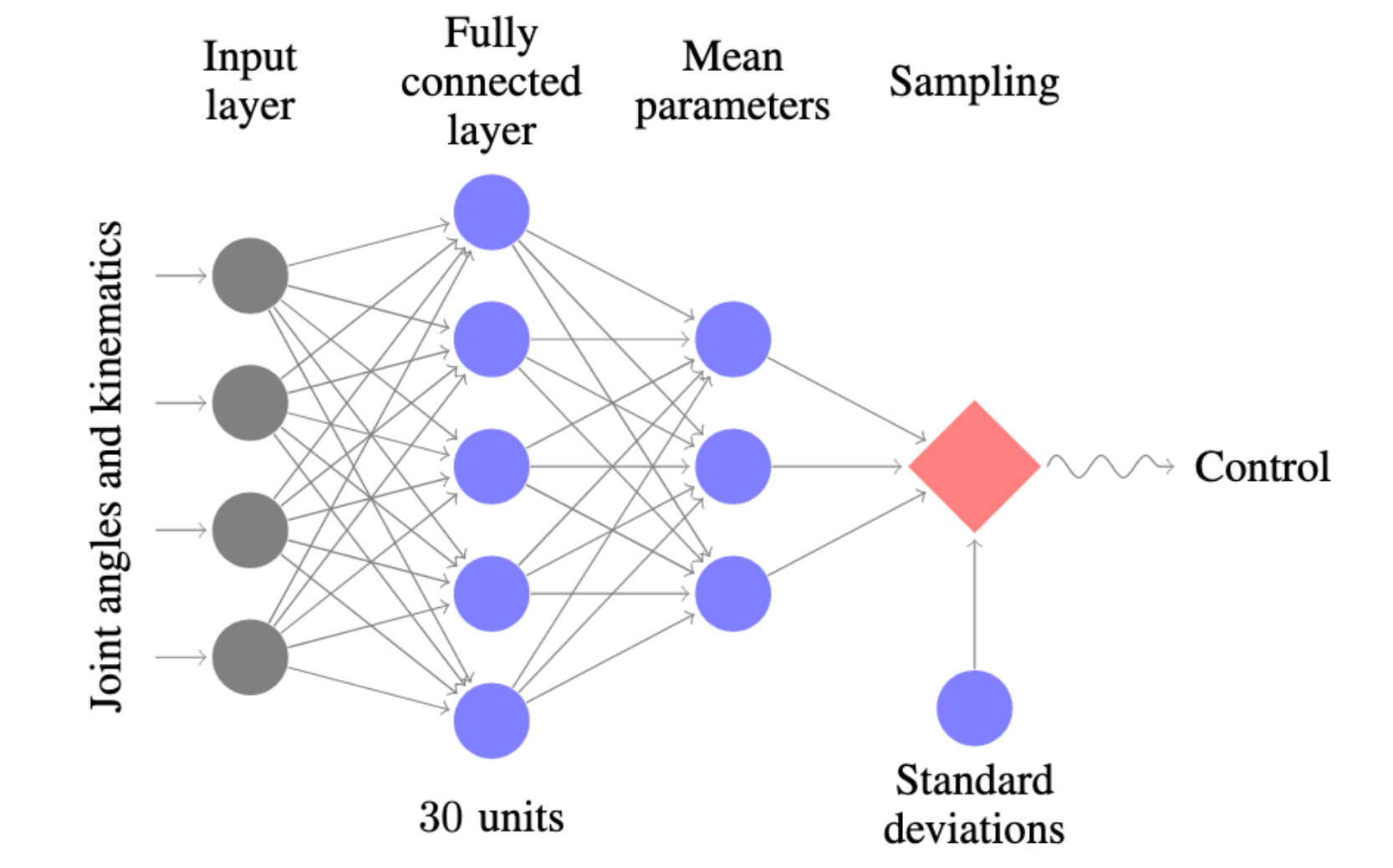
The correct mindset with a fully connected neural network is a depth of two or three, with the width set between 50 to 100 (or 64 to 128, if you want to fit in with the cool computer science folk). If your model is low bias, consider adding capacity through another layer or additional width.

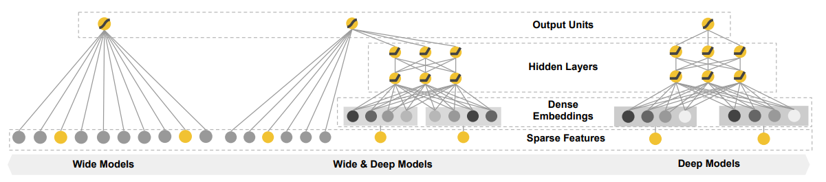
One interesting improvement on the simple fully connected architecture is the wide & deep architecture, which mixes wide memorization feature interactions with deep unseen, learned feature combinations.

Cheng et al. (2016) Wide & Deep Learning for Recommender Systems

PEP 8

Programs must be written for people to read, and only incidentally for machines to execute.

Abelson & Sussman - Structure and Interpretation of Computer Programs

Code style is important. I remember being confused at why more experienced programmers were so particular about code style.

After programming for five years, I now know where they were coming from.

Code that is laid out in the expected way requires less effort is required to read & understand code. Poor code style places additional burden on the reader to understand your unique code style, before they even think about the actual code itself.

#  bad
Var=1

def adder ( x =10 ,y= 5):
    return  x+y

#  good
var = 1

def adder(x=10, y=5):
    return x + y

All good text editors will have a way to integrate in-line linting - highlighting mistakes as you write them. Automatic, in-line linting is the best way to learn code style - take advantage of it.

Drop the Target

If you ever get a model with an impossibly perfect performance, it is likely that your target is a feature.

#  bad
data.drop('target', axis=1)

#  good
data = data.drop('target', axis=1)

We all do it once.

Scale the Target or Features

This is the advice I’ve given most when debugging machine learning projects. Whenever I see a high loss (higher that say 2 or 3), it’s a clear sign that the target has not been scaled to a reasonable range.

Scale matters because unscaled targets lead to large prediction errors, which mean large gradients and unstable learning.

By scaling, I mean either standardization:

standardized = (data - np.mean(data)) / np.std(data)

Or normalization:

normalized = (data - np.min(data)) / (np.max(data) - np.min(data))

Note that there is a lack of consistency between what these things are called - normalization is also often called min-max scaling, or even standardization!

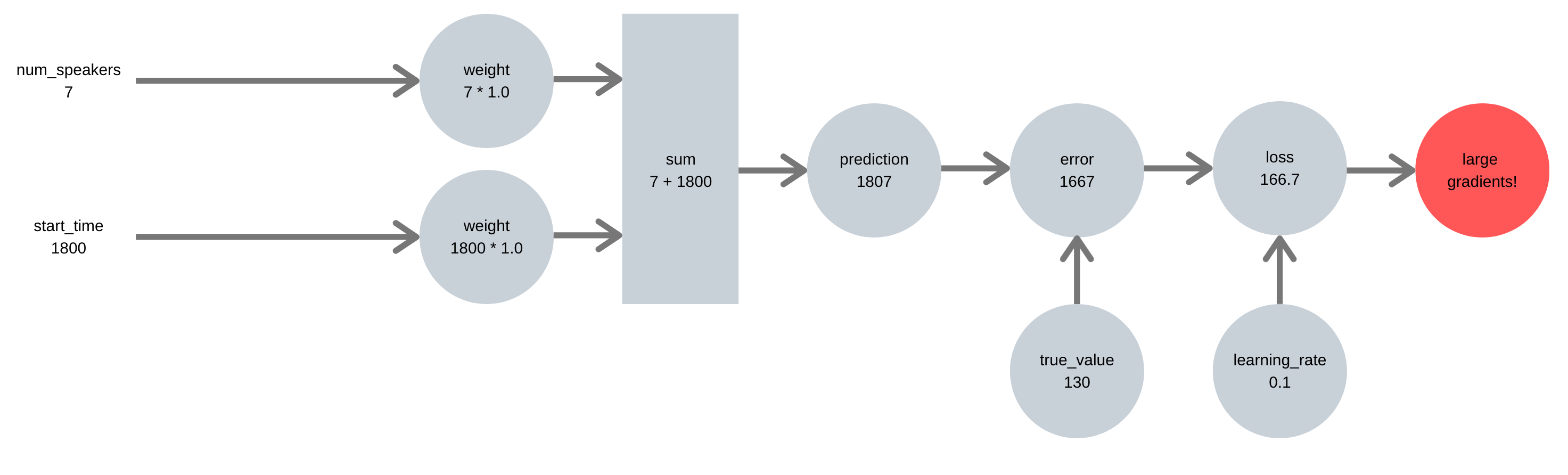
Take the example below, where we are trying to predict how many people attend a talk, from the number of speakers and the start time. Our first pipeline doesn’t scale the features or targets, leading to a large error signal and large gradients:

Our second pipeline takes the time to properly scale features & target, leading to an error signal with appropriately sized gradients:

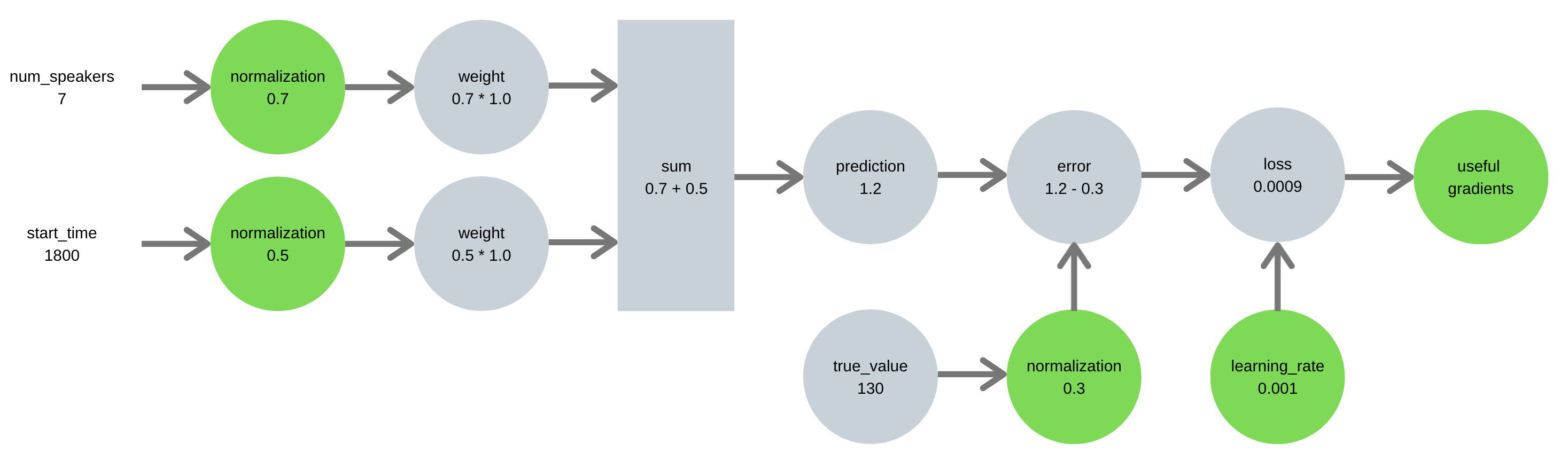
A similar logic holds for features - unscaled features can dominate and distort how information flows through a neural network.

Work with a Sample

This is a small workflow improvement that leads to massive productivity gains.

Development is a continual cycle of fixing errors, running code and fixing errors. Developing your program on a large dataset can cost you time - especially if your debugging something that happens at the end of the pipeline.

During development, work on a small subset of the data. There are a few ways to handle this.

Creating a Subset of the Data

You can work on a sample of your data already in memory, using an integer index:

data = data[:1000]

pandas allows you only load a subset of the data at a time (avoiding pulling the entire dataset into memory):

data = pd.read_csv('data.csv', nrows=1000)

Controlling the Debugging

A simple way to control this is a variable - this is what you would do in a Jupyter Notebook:

nrows = 1000
data = pd.read_csv('data.csv', nrows=nrows)

Or more cleanly with a command line argument:

#  data.py
parser.add_argument('--nrows', nargs='?')
args = parser.parse_args()
data = pd.read_csv('data.csv', nrows=args.nrows)
print(f'loaded {data.shape[0]} rows')

Which can be controlled when running the script data.py:

$ python data.py --nrows 1000

Don’t Write over Raw Data

Raw data is holy - it should never be overwritten. The results of any data cleaning should be saved separately to the raw data.

Use $HOME

This one is a pattern that has dramatically simplified my life.

Managing paths in Python can be tricky. There are few things that can change how path finding Python can work:

• where the user clones source code,
• where a virtual environment installs that source code,
• which directory a user runs a script from.

Some of the problems that occur are from these changes:

• os.path.realpath will change based on where the virtual environment installs your package,
• os.getcwd will change based on where the user runs Python the interpreter.

Putting data in a fixed, consistent place can avoid these issues - you don’t ever need to get the directory relative to anything except the users $HOME directory.

The solution is to create a folder in the user’s $HOME directory, and use it to store data:

import os

home = os.environ['HOME']
path = os.path.join(home, 'adg'))
os.makedirs(path, exist_ok=True)
np.save(path, data)

This means your work is portable - both to on your colleague’s laptops and on remote machines in the cloud.

---

Thanks for reading!