Typical Year Forecasting of Electricity Prices

Energy prices are volatile - the price of gas, oil and electricity can all change significantly year on year. Yet the energy industry ignores this year on year volatility when modelling investment decisions in energy projects.

This exposes projects to a significant source of hidden error in the form of variance in financial model results, leading to the wrong projects being built.

This post introduces a simple solution to this problem in the form of a typical year forecast.

You can find supporting materials for this work at adgefficiency/typical-year-forecasting-electricity-prices.

What is a Typical Year Forecast?

A typical year forecast uses historical data to create a single, synthetic year of data.

This single year forecast is suitable for use in business case modelling of energy projects - it’s not suitable for short term dispatch of energy assets.

A typical year forecast has the following advantages:

• simple to create - no machine learning, gradients or iterative calculations,
• interpretable - easy to understand why one sample is selected over others,
• realistic - the forecast is made from real historical data,
• domain flexible - can be used with any time series,
• statistically flexible - can use a range of statistics to define what typical means.

A typical year forecast has the following disadvantages:

• data quantity - requires at least 2 years of historical data,
• domain knowledge - requires selection & weighting of statistics.

An example of a typical year forecast is a typical metrological year (TMY) forecast, used to create a dataset of typical year of weather. TMY forecasts are commonly used in modelling solar generation or building energy use.

The idea & inspiration for this post came from using the TMY forecast produced by Solcast - thanks Solcast for the inspiration!

The Problem with the Standard Industry Approach

Estimating the economic performance (simple payback, IRR, NPV or rate of return on capital) of an investment in an energy project requires combining two models - a technical model and a financial model.

Commonly the technical model will model a single year in isolation, and is used as an input to the financial model.

The financial model will model multiple years over time (to model economic return over time), using the technical results as the basis for the first year with the financial inputs (such as prices) forecasted forward based on the single year technical results.

In the absence of forecasted energy prices across the future project lifetime, energy prices are often modelled in a similar way to the technical model - taking a single reference year of prices and forecasting them forward with assumptions of inflation.

A simple example of how a technical & financial model combine is given below:

• a technical model outputs annual savings of 150 MWh of electricity,
• we assume electricity prices at 100 $/MWh
• capital investment is estimated at $ 25,000.

The technical inputs & price assumptions are then forecast forward (here without inflation) to calculate cumulative savings:

year	capex	savings_mwh	price	savings_$	cumulative_savings_$
0	25000	150	100	15000	-10000
1	0	150	100	15000	5000
2	0	150	100	15000	20000
3	0	150	100	15000	35000

It’s not common to see both the project capex and savings in the same year (usually you need to build something before it gives a saving) - for this simple example please forgive this!

Why Using The Most Recent Prices is Wrong

Choosing the reference year for prices is commonly done by:

• taking the most recent prices,
• taking the most recent full calendar year of prices,
• taking the prices that align with the technical model.

If we were setting up our model in November 2022 with a technical model based on 2019 data, the standard industry approach would likely be one of the following:

• the most recent prices - October 2021 to September 2022,
• the most recent calendar year - January 2021 to December 2021,
• prices that align with the technical data - January 2019 to December 2019.

Below we will demonstrate why all of these commonly used methodologies introduce a large source of error.

Error of Using Recent Prices

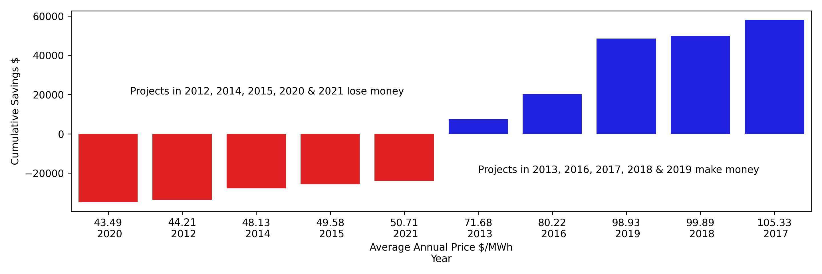
In our example above, we assumed prices at 100 $/MWh. The figure below uses the same financial model with the actual annual average electricity prices for South Australia:

Look at the variance of these results! Around half of our projects lose money, with the other half being profitable.

This variance error that the standard industry approaches are hiding - normally we only get a single estimate, without seeing the spread across different years of price data.

This variance in project performance is only occurring based on when we do our modelling - not based on the fundamental, underlying economics of the project.

We can do better!

Creating a Typical Year Forecast

Creating a typical year forecast requires defining what typical means.

For these forecasts we will define typical as similarity - our typical year forecast will be made of samples of data that are most similar to all the other data.

We can quantify similarity by defining an error metric - the error between statistics measured across all our data and statistics measured across a candidate sample. The samples that minimize this error will be selected and used in our forecast.

For our first typical year forecast, we will create a forecast based on a single statistic - the average price within a month.

The basic idea is as follows:

#  Creating a Typical Year Forecast based on the Mean with 5 Years of Historical Data.

#  Iterate across each month in a year (12 months in total).
for each month in a year (Jan, Feb ... Nov, Dec)
 
  #  Calculate one long term statistic across all 5 years for this one month.
  long_term_mean = historical_data[month].mean()

  #  Iterate across our historical data, selecting this one month,
  #  5 months across 5 years, all the same month.
  for year in historical_data
    sample_mean = year[month].mean()

    #  Calculate the error of this month versus the long term statistic.
    sample_error = absolute(sample_mean - long_term_mean)

  #  Select the sample with the lowest sample error,
  #  this is the historical month we will use in our typical year forecast.
  selected_sample = argmin(sample_errors)

After following this procedure, we will select 12 monthly samples - one for each month in a year, creating our typical year forecast.

Typical Year Forecast for South Australian Electricity Prices

To further demonstrate the idea, we will first limit ourselves to forecasting a single month - January, for electricity prices in South Australia, using 10 years of historical data.

Let’s first start by calculating our long term statistic - the average price in January across the entire dataset, which is 85.449 $/MWh.

We can then look at what the average price was in each January and calculate the error versus the long term statistic.

This leads us to selecting January 2017 as our typical month of electricity prices:

year	month	price-mean	long-term-mean	error-mean
2012	January	25.6153	85.449	59.8337
2013	January	59.1246	85.449	26.3244
2014	January	88.8675	85.449	3.41845
2015	January	34.68	85.449	50.769
2016	January	50.2573	85.449	35.1917
2017	January	84.2589	85.449	1.19009
2018	January	158.757	85.449	73.3081
2019	January	241.025	85.449	155.576
2020	January	83.2037	85.449	2.24526
2021	January	28.7008	85.449	56.7482

We can then repeat the procedure above to forecast the remaining 11 months of the year, ending up with 12 months that make up our typical year forecast:

year	month	price-mean	long-term-mean	error-mean
2017	January	84.2589	85.449	1.19009
2020	February	64.1771	71.2239	7.04685
2021	March	68.7727	66.6858	2.08692
2021	April	52.1361	64.1214	11.9854
2016	May	70.6976	70.1316	0.565976
2021	June	84.3886	81.6753	2.71335
2021	July	91.1873	94.7737	3.58638
2016	August	66.2397	64.8625	1.37717
2012	September	53.7977	54.7594	0.961707
2012	October	50.9616	52.3186	1.35705
2016	November	61.8883	57.3279	4.56045
2015	December	66.8321	67.2765	0.444369

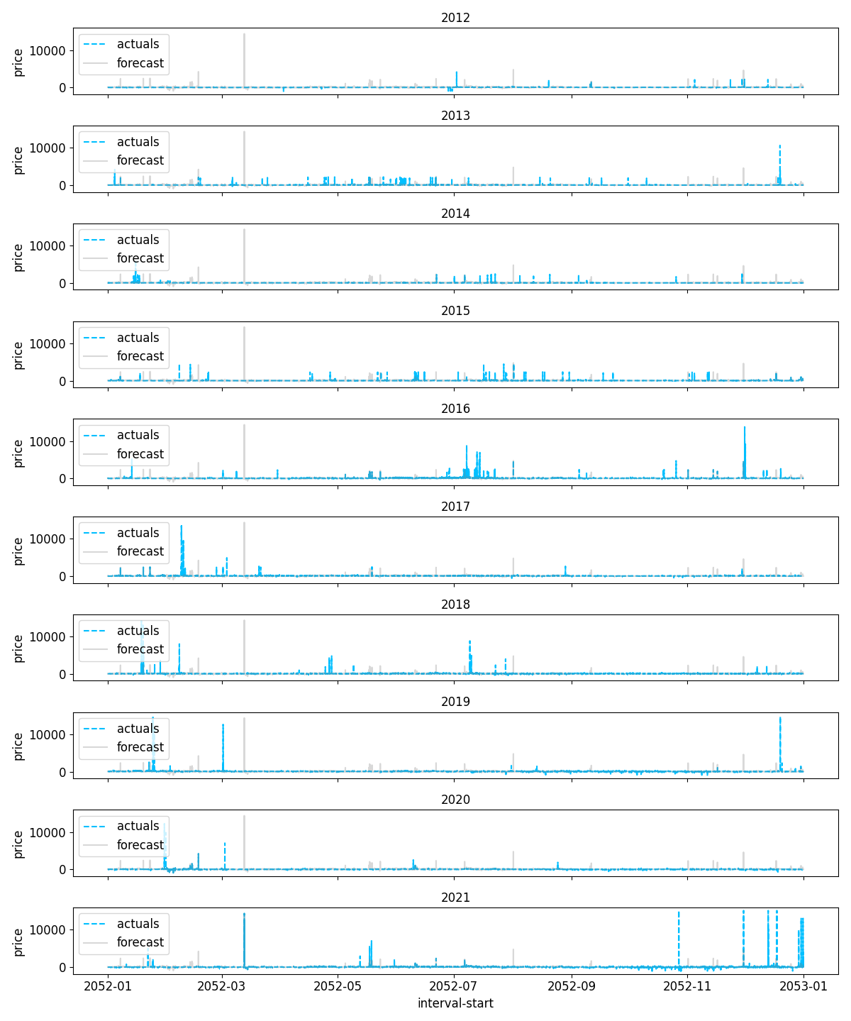
Our typical year forecast, in all it’s light blue glory:

We can compare this typical year forecast to actual historical prices - for the years where we have sampled our typical month from, our forecast directly overlaps the historical data:

Extending the Forecast With More Statistics

Above we only considered the mean when selecting a month. The mean is a measurement of the central tendency of a distribution - using the mean to select a month will mean our forecast has a similar central point to the long term average.

For some energy models, the variance is more important than the average.

The variance is how spread out prices are - it’s important for batteries operating in wholesale arbitrage, as this spread puts an upper limit on the profitability of shifting of electricity between intervals can be.

Our procedure for creating a typical year forecast based on both the mean and the variance is similar to only considering the mean.

We instead calculate two additional statistics (the long term standard deviation and the sample standard deviation), and include them in our sample error:

#  Creating a typical year forecast based on the mean & standard deviation

#  Iterate across each month in a year.
for month in (Jan, Feb ... Nov, Dec):

  #  Calculate two statistics - long term mean & standard deviation.
  long_term_mean = data.mean()
  long_term_std = data.std()

  #  Iterate across historical data & calculate sample errors,
  #  using both long term statistics
  for year in (historical data):
    sample_mean = month.year.mean()
    sample_std = month.year.std()
    sample_error = absolute(long_term_mean - sample_mean) + absolute(long_term_std - sample_std)

  #  Select sample that minimizes error.
  selected_sample = argmin(sample_errors)

Taking this approach again, we end up with our typical year forecast - different from our previous forecast where we only used the mean:

month	year	price-mean	long-term-mean	price-std	long-term-std	error
January	2020	83.2037	85.449	519.785	504.705	17.3251
February	2018	109.17	71.2239	290.873	300.955	48.0282
March	2020	46.9517	66.6858	225.829	271.301	65.2057
April	2015	39.9493	64.1214	100.387	99.2508	25.3085
May	2016	70.6976	70.1316	132.686	133.63	1.5091
June	2021	84.3886	81.6753	96.1186	130.305	36.8999
July	2015	73.5053	94.7737	226.191	236.491	31.5684
August	2013	71.2364	64.8625	88.1036	103.648	21.9185
September	2012	53.7977	54.7594	62.1015	75.617	14.4772
October	2019	67.3398	52.3186	92.2279	108.001	30.7947
November	2019	50.8623	57.3279	88.3317	109.014	27.1474
December	2013	79.5734	67.2765	372.848	318.756	66.3892

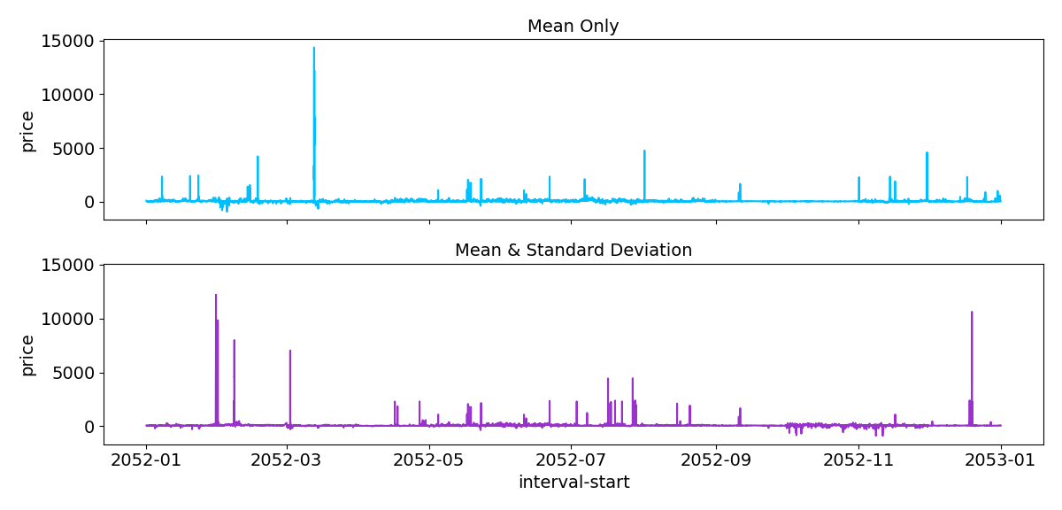
We can compare our two typical year forecasts directly:

Typical year forecasting based on both the mean and the variance is selecting months with higher prices - including more of the tasty price spikes that makes Australia’s National Electricity Market (NEM) so interesting for battery storage.

Evaluating the Typical Year Forecast

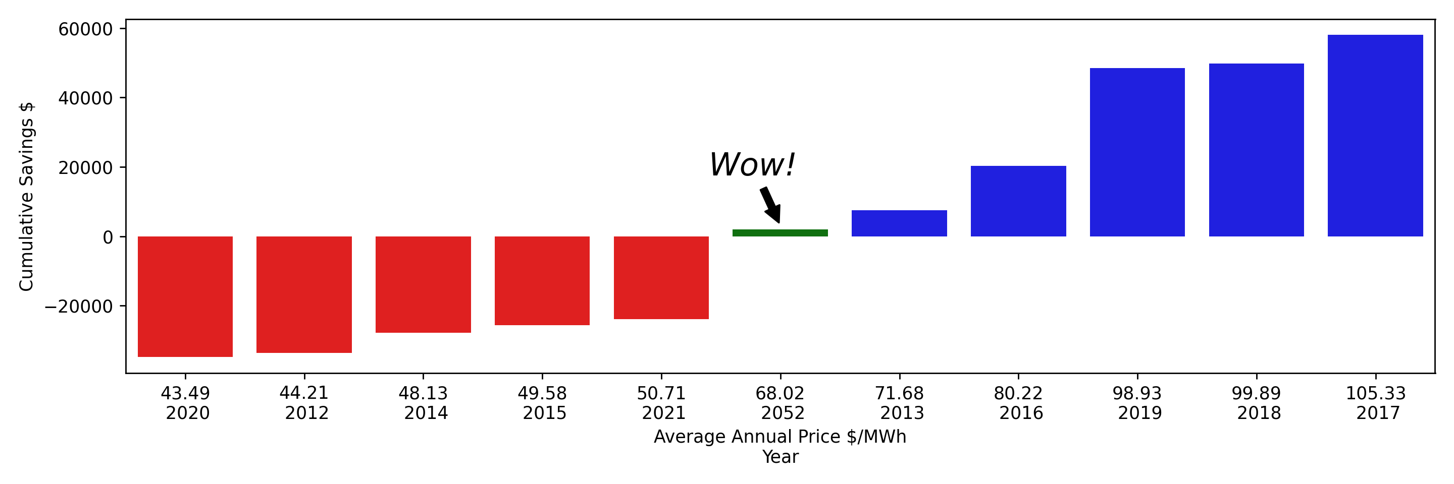
Let’s return to our original motivating example, with an additional estimate of our project cumulative savings using our typical year forecast based on using the mean (show as 2052 in green):

How great is that!

Our typical year forecast does a fantastic job of cutting through the variance - modelling our project right in the middle of the high variance estimates we get when taking the traditional, industry standard approaches of using historical price data.

No longer are we slaves to the cruel master of time (well, perhaps we still are) - as the years go by, our estimation of project economics will stay stable and consistent, rather than varying wildly based on when we are doing our modelling.

As new price data becomes available, our typical year forecast will change (due to both the long term statistics changing, or recent data being more typical), but the variance from these changes will be minor compared to the massive year on year swings we get with the standard industry approaches.

Discussion

Above we have seen how great our typical year forecast is at reducing the variance of our estimates of project performance - let’s now discuss some challenges and potential extensions to this simple typical year forecasting method.

Challenges

Data Quantity

This methodology requires multiple years of data - if we only have access to a single year, this method is not appropriate.

Alignment

One problem that arises when concatenating interval data from different time periods together is alignment at the intersection - the sample below from the typical year forecast produced above shows the issue - our forecast jumps from Tuesday in January 2017 to Friday 2020:

forecast	original-timestamps	price	day-of-week-forecast	day-of-week-original
2052-01-31 23:50:00	2017-01-31 23:50:00	39.52	2	1
2052-01-31 23:55:00	2017-01-31 23:55:00	39.52	2	1
2052-02-01 00:00:00	2020-02-01 00:00:00	299.2	3	5
2052-02-01 00:05:00	2020-02-01 00:05:00	299.2	3	5

This misalignment will cause issues with the incorrect number of weekdays or weekends in a year - important as energy demand and price has strong weekly seasonality.

This alignment problem also occurs when you don’t use a typical year forecast - for example if you use price data from 2022 with technical data from 2010.

Domain Expertise

Domain expertise is required to setup a typical year forecast - primarily in defining the appropriate statistics.

Using multiple statistics can also require weighting - for example if the standard deviation is orders of magnitude higher than the mean, we may want to weight the mean higher.

Extensions & Improvements

Higher Frequency Sampling

In the examples above we have selected samples on a monthly basis - it is possible to instead select samples on a different frequency, such as week of the year (52 weeks) or day of the year (365 days).

More Statistics

One advantage of this methodology are flexibility of statistics we choose - unlike a loss function for a neural network, they do not need to be differentiable.

For example, we could use statistics like:

• mean, median, mode,
• number of time periods above a threshold price,
• number of negative prices.

This is an exciting feature of typical year forecasting - the flexibility and simplicity of using any statistic that aligns with what your technical and financial models need to align with your business goals.

Summary

In this post we introduced typical year forecasting - a flexible, powerful forecasting method suitable for use in energy project business case modelling.

Typical year forecast address a hidden flaw in the price assumptions commonly used in industry - the large errors introduced by using recent price data.

A typical year forecast addresses these issues by selecting historical price data that is most similar to all the historical data.

Typical year forecasts have the following advantages:

• simple to create - no machine learning, gradients or iterative calculations,
• interpretable - easy to understand why one sample is selected over others,
• realistic - the forecast is made from actual historical data,
• domain flexible - can be used with any time series (not just electricity prices),
• statistically flexible - can use a range of statistics to define what typical means.

A typical year forecast has the following disadvantages:

• data quantity - requires at least 2 years of historical data,
• domain knowledge - requires selecting & weighting of statistics based on problem understanding.

Further extensions on the methods shown above include:

• higher frequency sampling on a weekly or daily basis,
• using a variety of statistics to define similarity, such as the number of price spikes or the number of negative prices.

---

Thanks for reading!

If you enjoyed this post, make sure to check out Measuring Forecast Quality using Linear Programming.

You can find the materials to reproduce this analysis at adgefficiency/typical-year-electricity-price-forecasting.