A Guide to Deep Learning Layers

Summary

Layer	Intuition	Inductive Bias	When To Use
Fully connected	Allow all possible connections	None	Data without structure (tabular data)
2D convolution	Recognizing spatial patterns	Local, spatial patterns	Data with spatial structure (images)
LSTM	Database	Sequences & memory	Never - use Attention
Attention	Focus on similarities	Similarity & limit information flow	Data with sequential structure

Introduction

This post is about four fundamental neural network layer architectures - the building blocks that machine learning engineers use to construct deep learning models.

The four layers are:

1. the fully connected layer,
2. the 2D convolutional layer,
3. the LSTM layer,
4. the attention layer.

For each layer we will look at:

• how each layer works,
• the intuition behind each layer,
• the inductive bias of each layer,
• what the important hyperparameters are for each layer,
• when to use each layer,
• how to program each layer in TensorFlow 2.0.

All code examples are built using tensorflow==2.2.0 using the Keras Functional API.

Background - what is inductive bias?

A key term in this article is inductive bias - a useful term to sound clever and impress your friends.

Inductive bias is the hard-coding of assumptions into the structure of a learning algorithm. These assumptions make the method more special purpose, less flexible but more useful. By hard coding in assumptions about the structure of the data & task, we can learn functions that we otherwise can’t.

Examples of inductive bias in machine learning include margin maximization (classes should be separated by as large a boundary as possible - used in Support Vector Machines) and nearest neighbours (samples close together in feature space are in the same class - used in the k-nearest neighbours algorithm).

A bit of bias is good - this is a common lesson in machine learning (bias can be traded off for variance). This also holds in reinforcement learning, where unbiased approxmiations of a high variance Monte Carlo return performs worse than bootstrapped temporal difference methods.

1. The Fully Connected Layer

The fully connected layer is the most general purpose deep learning layer.

Also known as a dense or feed-forward layer, this layer imposes the least amount of structure of our layers. It will be found in almost all neural networks - if only used to control the size & shape of the output layer.

How does the fully connected layer work?

At the heart of the fully connected layer is the artificial neuron - the distant ancestor of McCulloch & Pitt’s Threshold Logic Unit of 1943.

The artificial neuron is inspired by the biological neurons in our brains - however an artificial neuron is a shallow approximation of the complexity of a biological neuron.

The artificial neuron composed of three sequential steps:

1. weighted linear combination of inputs,
2. sum across weighted inputs,
3. activation function.

1. Weighted linear combination of inputs

The strength of the connection between nodes in different layers are controlled by weights - the shape of these weights depending on the number of nodes layers on either side. Each node has an additional parameter known as a bias, which can be used to shift the output of the node independently of it’s input.

The weights and biases are learnt - commonly in modern machine learning backpropagation is used to find good values of these weights - good values being those that lead to good predictive accuracy of the network on unseen data.

2. Sum across all weighted inputs

After applying the weight and bias, all of the inputs into the neuron are summed together to a single number.

3. Activation function

This is then passed through an activation function. The most important activation functions are:

• linear activation function - unchanged output,
• ReLu - $0$ if the input is negative, otherwise input is unchanged
• Sigmoid squashes the input to the range $(0, 1)$
• Tanh squashes the input to the range $(-1, 1)$

The output of the activation function is input to all neurons (also known as nodes or units) in the next layer.

This is where the fully connected layer gets it’s name from - each node is fully connected to the nodes in the layers before & after it.

A single neuron with a ReLu activation function

For the first layer, the node gets it’s input from the data being fed into the network (each data point is connected to each node). For last layer, the output is the prediction of the network.

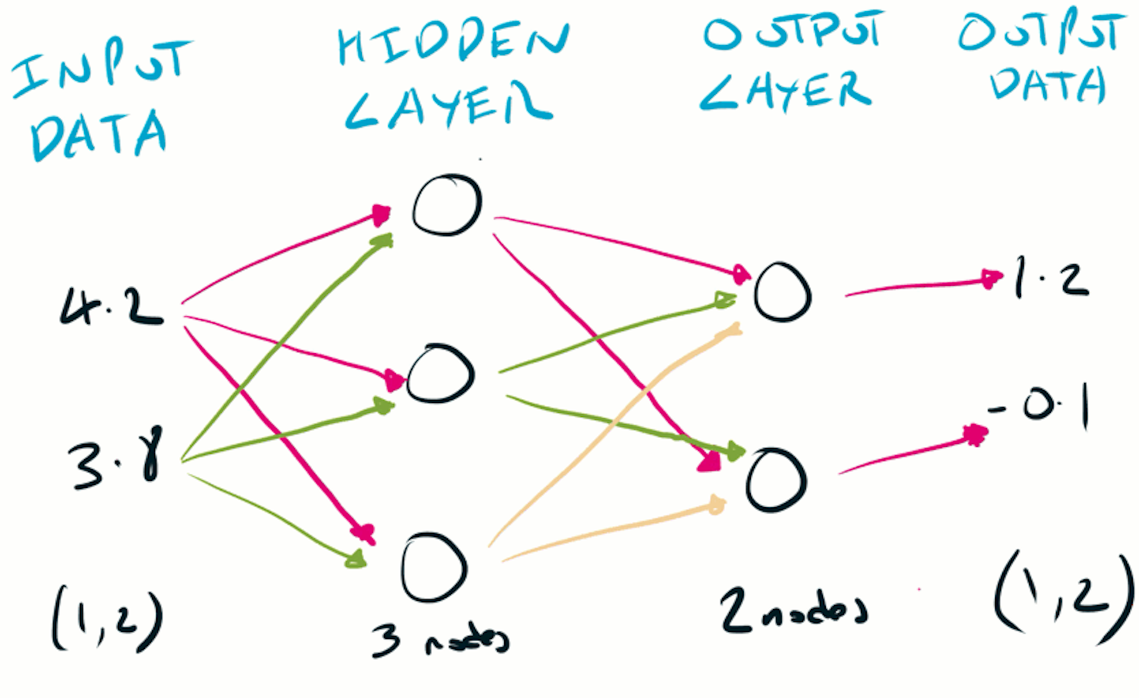
The fully connected layer

What is the intuition & inductive bias of a fully connected layer?

The intuition behind all the connections in a fully connected layer is to put no restriction on information flow. It’s the intuition of having no intuition.

The fully connected layer imposes no structure and makes no assumptions about the data or task the network will perform. A neural network built of fully connected layers can be thought of as a blank canvas - impose no structure and let the network figure everything out.

Universal Approximation (Except in Practice)

This lack of structure is what gives neural networks of fully connected layers (of sufficient depth & width) the ability to approximate any function - known as the Universal Approximation Theorem.

The ability to learn any function at first sounds attractive. Why do we need any other architecture if a fully connected layer can learn anything?

Being able to learn in theory does not mean we can learn in practice. Actually finding the correct weights, using the data and learning algorithms (such as backpropagation) we have available may be impractical and unreachable.

The solution to these practical challenges is to use less specialized layers - layers that have assumptions about the data & task they are expected to perform. This specialization is their inductive bias.

When should I use a fully connected layer?

A fully connected layer is the most general deep learning architecture - it imposes no constraints on the connectivity of each laver.

Use it when your data has no structure that you can take advantage of - if your data is a flat array (common in tabular data problems), then a fully connected layer is a good choice. Most neural networks will have fully connected layers somewhere.

Fully connected layers are common in reinforcement learning when learning from a flat environment observation.

For example, a network with a single fully connected layer is used in the Trust Region Policy Optimization (TRPO) paper from 2015:

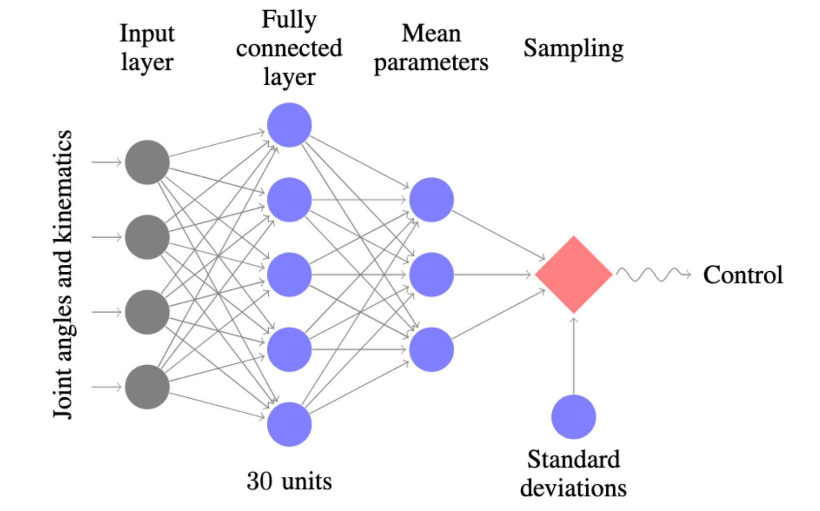
A fully connected layer being used to power the reinforcement learning algorithm TRPO

Fully connected layers are common as the penultimate & final layer as fully connected on convolutional neural networks performing classification. The number of units in the fully connected output layer will be equal to the number of classes, with a softmax activation function used to create a distribution over classes.

What hyperparameters are important for a fully connected layer?

The two hyperparameters you’ll often set in a fully connected layer are the:

1. number of nodes,
2. activation function.

A fully connected layer is defined by a number of nodes (also known as units), each with an activation function. While you could have a layer with different activation functions on different nodes, most of the time each node in a layer has the same activation function.

For hidden layers, the most common choice of activation function is the rectified-linear unit (the ReLu). For the output layer, the correct activation function depends on what the network is predicting:

• regression, target can be positive or negative -> linear (no activation),
• regression, target can be positive only -> ReLu,
• classification -> Softmax,
• control action, bound between -1 & 1 -> Tanh.

Using fully connected layers with the Keras Functional API

Below is an example of how to use a fully connected layer with the Keras functional API.

We are using input data shaped like an image, to show the flexibility of the fully connected layer - this requires us to use a Flatten layer later in the network:

import numpy as np
import tensorflow as tf
from tensorflow.keras import Input, Model
from tensorflow.keras.layers import Dense, Flatten

#  the least random of all random seeds
np.random.seed(42)
tf.random.set_seed(42)

#  dataset of 4 samples, 32x32 with 3 channels
x = np.random.rand(4, 32, 32, 3)

inp = Input(shape=x.shape[1:])
hidden = Dense(8, activation='relu')(inp)
flat = Flatten()(hidden)
out = Dense(2)(flat)
mdl = Model(inputs=inp, outputs=out)

mdl(x)
"""
<tf.Tensor: shape=(4, 2), dtype=float32, numpy=
array([[ 0.23494382, -0.40392348],
       [ 0.10658629, -0.31808627],
       [ 0.42371386, -0.46299127],
       [ 0.34416917, -0.11493915]], dtype=float32)>
"""

2. The 2D Convolutional Layer

If you had to pick one architecture as the most important in deep learning, it’s hard to look past convolution (see what I did there?).

The winner of the 2012 ImageNet competition, AlexNet, is seen by many as the start of modern deep learning. Alexnet was a deep convolutional neural network, trained on GPU to classify images.

Another landmark use of convolution is Le-Net-5 in 1998, a 7 layer convolutional neural network developed by Yann LeCun to classify handwritten digits.

The convolutional neural network is the original workhorse of the modern deep learning revolution - it can be used with text, audio, video and images.

Convolutional neural networks can be used to classify the contents of the image, recognize faces and create captions for images. They are also easy to parallelize on GPU - making them fast to train.

What is the intuition and inductive bias of convolutional layers?

Convolution itself is a mathematical operation, commonly used in signal processing. The 2D convolutional layer is inspired by our own visual cortex.

The history of using convolution in artificial neural networks goes back decades to the neocognitron, an architecture introduced by Kunihiko Fukushima in 1980, inspired by the work of Hubel & Wiesel.

Work by the neurophysiologists Hubel & Wiesel in the 1950’s showed that individual neurons in the visual cortexes of mammals are activated by small regions of vision.

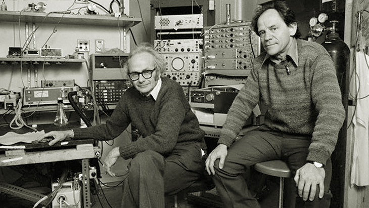
Hubel & Wiesel

A good mental model for convolution is the process of sliding a filter over a signal, at each point checking to see how well the filter matches the signal.

This checking process is pattern recognition, and is the intuition behind convolution - looking for small, spatial patterns anywhere in a larger space. The convolution layer has inductive bias for recognizing local, spatial patterns.

How does a 2D convolution layer work?

A 2D convolutional layer is defined by the interaction between two components:

1. a 3D image, with shape (height, width, color channels),
2. a 2D filter, with shape (height, width).

The intuition of convolution is looking for patterns in a larger space.

In a 2D convolutional layer, the patterns we are looking for are filters, and the larger space is an image.

Filters

A convolutional layer is defined by it’s filters. These filters are learnt - they are equivalent to the weights of a fully connected layer.

Filters in the first layers of a convolutional neural network detect simple features such as lines or edges. Deeper in the network, filters can detect more complex features that help the network perform it’s task.

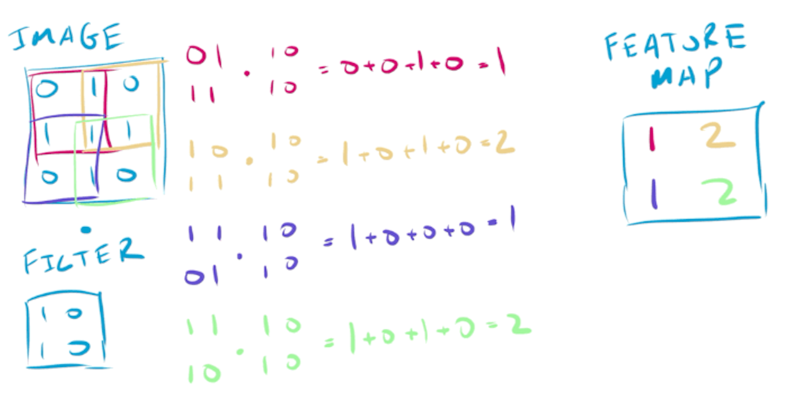
To further understand how these filters work, let’s work with a small image and two filters. The basic operation in a convolutional neural network is to use these filters to detect patterns in the image, by performing element-wise multiplication and summing the result:

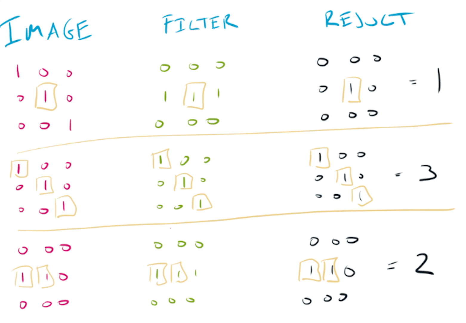
Applying different filters to a small image

Reusing the same filters over the entire image allows features to be detected in any part of the image - a property known as translation invariance. This property is ideal for classification - you want to detect a cat no matter where it occurs in the image.

For larger images (which are often 32x32 or larger), this same basic operation is performed, with the filter being passed over the entire image. The output of this operation acts as feature detection, for the filters that the network has learnt, producing a 2D feature map.

A filter producing a filter map by convolving over an image

The feature maps produced by each filter are concatenated, resulting in a 3D volume (the length of the third dimension being the number of filters).

The next layer then performs convolution over this new volume, using a new set of learned filters.

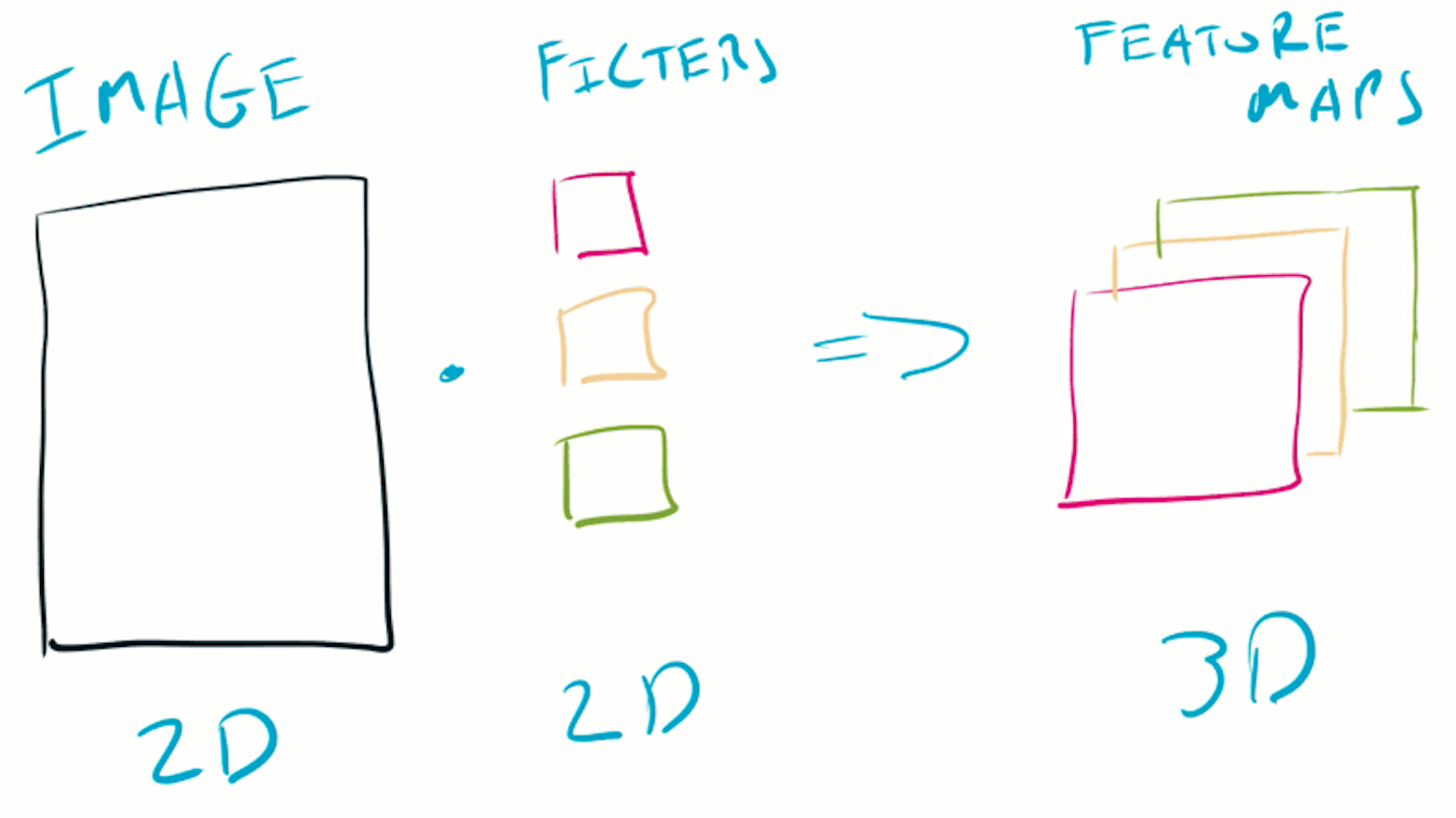
The feature maps of multiple filters are concatenated to produce a volume, which is passed to the next layer.

2D convolutional neural network built using the Keras Functional API

Below is an example of how to use a 2D convolution layer with the Keras functional API:

• the Flatten layer before the dense layer, to flatten our volume produced by the 2D convolutional layer,
• the Dense layer size of 8 - this controls how many classes our network can predict.

import numpy as np
import tensorflow as tf
from tensorflow.keras import Input, Model
from tensorflow.keras.layers import Dense, Flatten, Conv2D

np.random.seed(42)
tf.random.set_seed(42)

#  dataset of 4 images, 32x32 with 3 color channels
x = np.random.rand(4, 32, 32, 3)

inp = Input(shape=x.shape[1:])
conv = Conv2D(filters=8, kernel_size=(3, 3), activation='relu')(inp)
flat = Flatten()(conv)
feature_map = Dense(8, activation='relu')(flat)
out = Dense(2, activation='softmax')(flat)
mdl = Model(inputs=inp, outputs=out)

mdl(x)
"""
<tf.Tensor: shape=(4, 2), dtype=float32, numpy=
array([[-0.39803684, -0.08939186],
       [-0.48165476, -0.28876644],
       [-0.32680377, -0.24380796],
       [-0.45394567, -0.28233868]], dtype=float32)>
"""

What hyperparameters are important for a convolutional layer?

The important hyperparameters in a convolutional layer are:

• the number of filters,
• filter size,
• activation function,
• strides,
• padding,
• dilation rate.

The number of filters determines how many patterns each layer can learn. It’s common to have the number of filters increasing with the depth of the network. Filter size is commonly set to (3, 3), with a ReLu as the activation function.

Strides can be used to skip steps in the convolution, resulting in smaller feature maps. Padding allows pixels on the edge of the image to act as if they are in the middle of an image. Dilation allow the filters to operate over a larger area of the image, while still producing feature maps of the same size.

When should I use a convolutional layer?

Convolution works when your data has a spatial structure - for example, images have spatial structure in height & width. You can also get this structure from a 1D signal using techniques such as Fourier Transforms, and then perform convolution in the frequency domain.

If you are working with images, convolution is king. While there is work applying attention based models to computer vision, because of it’s similarity with our own visual cortex, it is likely that convolution will be relevant for many years to come.

An example of using convolution occurs in DeepMind’s 2015 DQN work. The agent learns to take decisions using pixels - making convolution a strong choice:

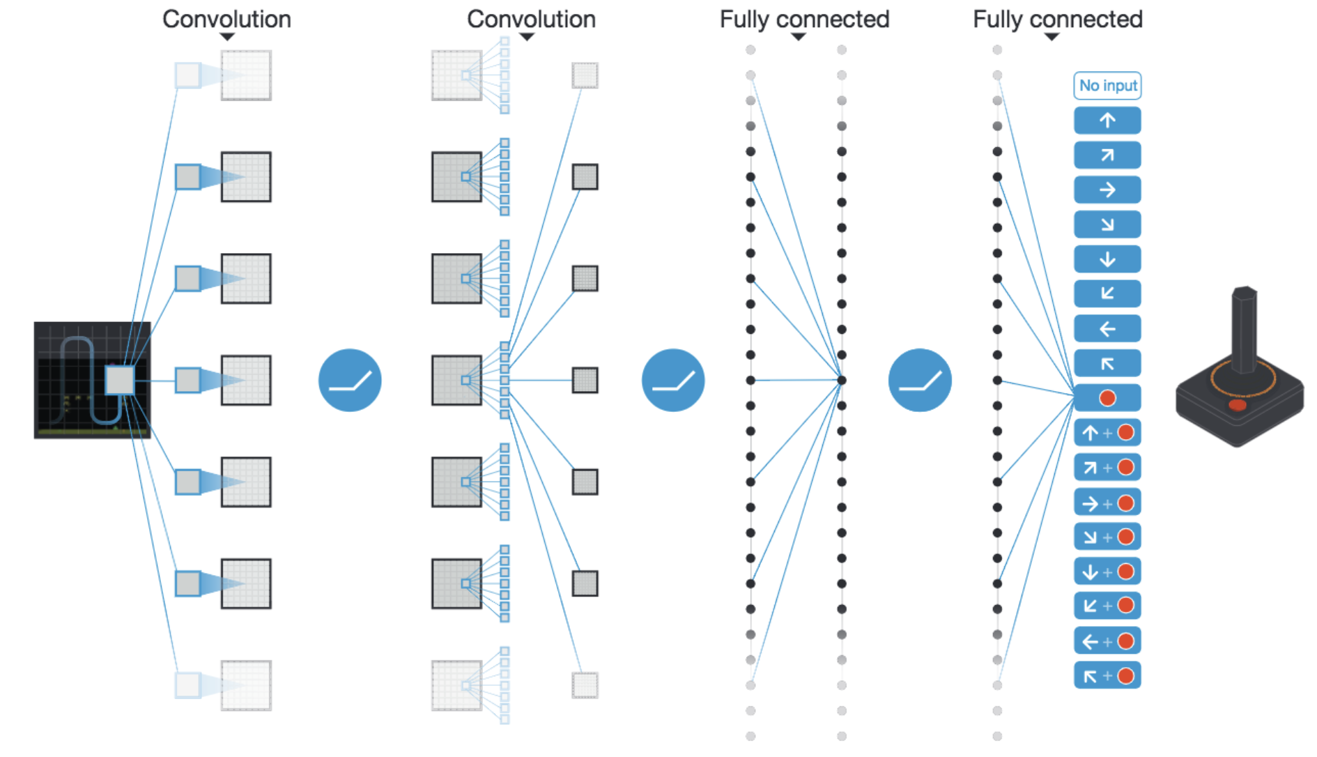
Deep convolutional neural network used in the 2015 DeepMind DQN Atari work

So what other kinds of structure can data have, other than spatial? Many types of data have a sequential structure - motivating our next two layer architectures.

3. LSTM Layer

The third of our layers is the LSTM, or Long Short-Term Memory layer. The LSTM is recurrent and processes data as a sequence.

Recurrence allows a network to experience the temporal structure of data, such as words in a sentence, or time of day.

A normal neural network receives a single input tensor $x$ and generates a single output tensor $y$. A recurrent architecture differs from a non-recurrent neural network in two ways:

1. both the input $x$ & output $y$ data is processed as a sequence of timesteps,
2. the network has the ability to remember information and pass it to the next timestep.

The memory of a recurrent architecture is known as the hidden state $h$. What the network chooses to pass forward in the hidden state is learnt by the network.

A recurrent neural network

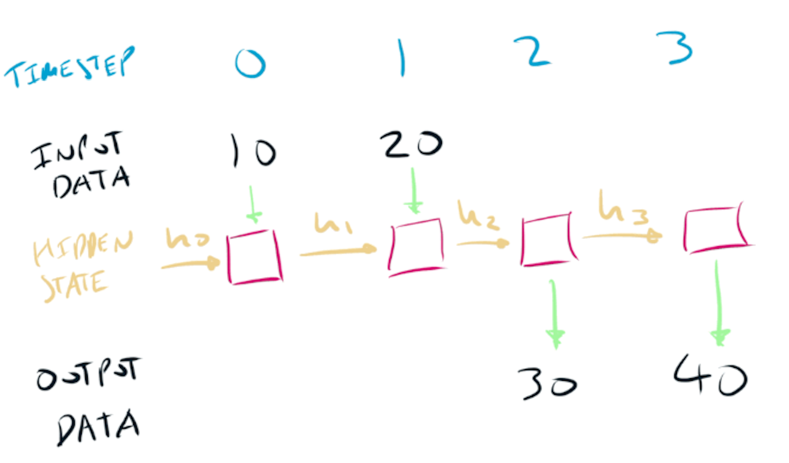
Entering the timestep dimension

Working with recurrent architectures requires being comfortable with the idea of a timestep dimension - knowing how to shape your data correctly is half the battle of working with recurrence.

Imagine we have input data $x$, that is a sequence of integers [0, 0] -> [2, 20] -> [4, 40]. If we were using a fully connected layer, we could present this data to the network as a flat array:

import numpy as np

x = np.zeros(10).astype(int)
x[0::2] = np.arange(0, 10, 2)
x[1::2] = np.arange(0, 100, 20)
x = x.reshape(1, -1)

print(x)
# array([[ 0,  0,  2, 20,  4, 40,  6, 60,  8, 80]])

print(x.shape)
# (1, 10)

Although the sequence is obvious to us, it’s not obvious to a fully connected layer.

All a fully connected layer would see is a list of numbers - the sequential structure would need to be learnt by the network.

We can restructure our data $x$ to explicitly model this sequential structure, by adding a timestep dimension. The values in our data do not change - only the shape changes:

import numpy as np

x = np.vstack([np.arange(0, 10, 2), np.arange(0, 100, 20)]).T
x = x.reshape(1, 5, 2)
print(x)
"""
array([[[ 0,  0],
        [ 2, 20],
        [ 4, 40],
        [ 6, 60],
        [ 8, 80]]])
"""

print(x.shape)
# (1, 5, 2)

Our data $x$ is now structured with three dimensions - (batch, timesteps, features). A recurrent neural network will process the features one timestep at a time, experiencing the sequential structure of the data.

Now that we understand how to structure data to be used with a recurrent neural network, we can take a high-level look at details of how the LSTM layer works.

How does an LSTM layer work?

The LSTM was first introduced in 1997 and has formed the backbone of modern sequence based deep learning models, excelling on challenging tasks such as machine translation. For years the state of the art in machine translation was the seq2seq model, which is powered by the LSTM.

The LSTM is a specific type a recurrent neural network. The LSTM addresses a challenge that vanilla recurrent neural networks struggled with - the ability to think long term.

In a recurrent neural network all information passed to the next time step has to fit in a single channel, the hidden state $h$.

The LSTM addresses the long term memory problem by using two hidden states, known as the hidden state $h$ and the cell state $c$. Having two channels allows the LSTM to remember on both a long and short term.

Internally the LSTM makes use of three gates to control the flow of information:

1. forget gate to determine what information to delete,
2. input gate to determine what to remember,
3. output gate to determine what to predict.

One important architecture that uses LSTMs is seq2seq. The source sentence is fed through an encoder LSTM to generate a fixed length context vector. A second decoder LSTM takes this contex vector and generates the target sentence.

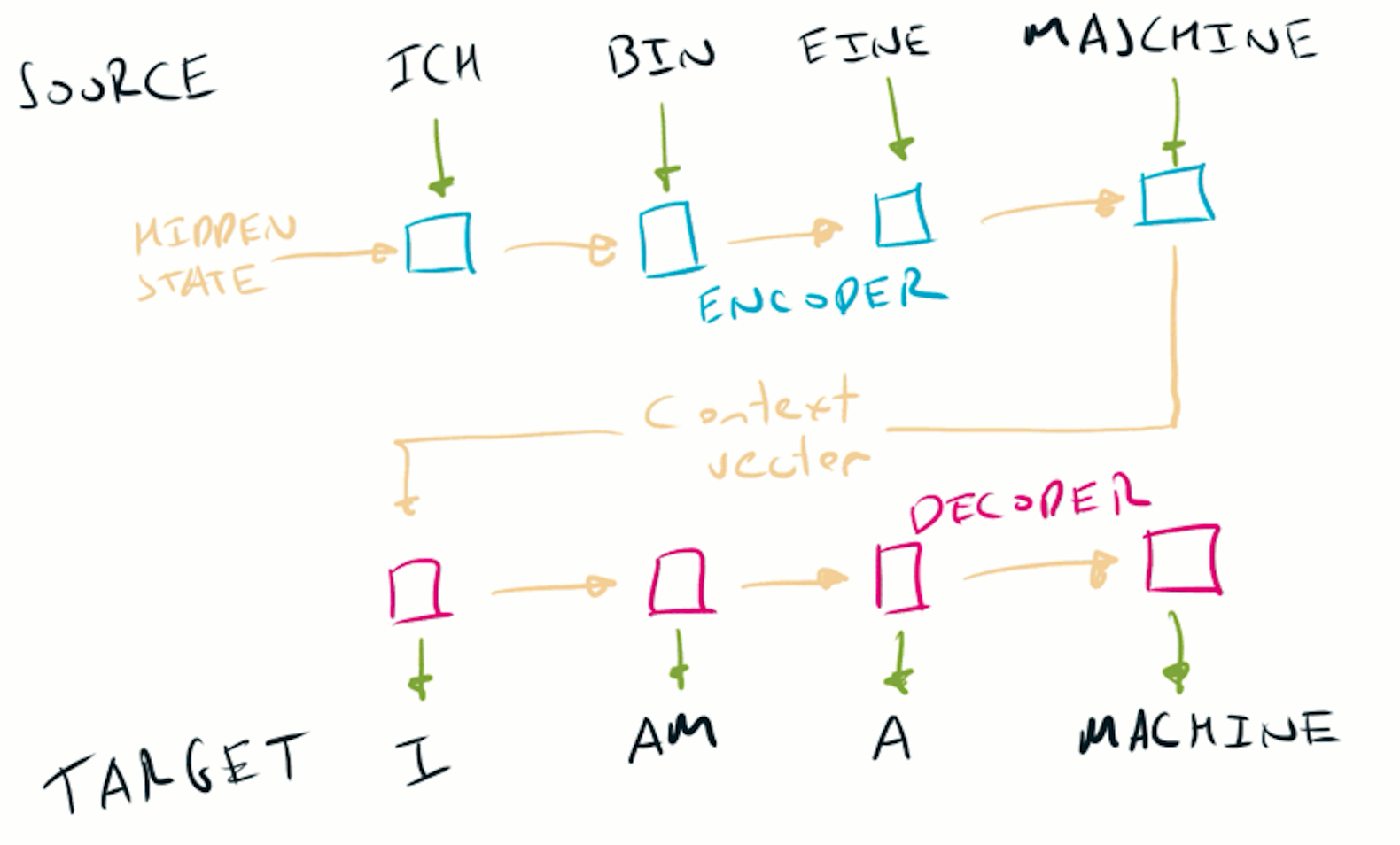
The seq2seq model

For a deeper look at the internal of the LSTM, take a look at the excellent Understanding LSTM Networks from colah’s blog.

What is the intuition and inductive bias of an LSTM?

A good intiutive model for the LSTM layer is to think about it like a database. The output, input and delete gates allow the LSTM to work like a database - matching the GET, POST & DELETE of a REST API, or the read-update-delete operations of a CRUD application.

The forget gate acts like a DELETE, allowing the LSTM to remove information that isn’t useful. The input gate acts like a POST, where the LSTM can choose information to remember. The output gate acts like a GET, where the LSTM chooses what to send back to a user request for information.

A recurrent neural network has has an inductive bias for processing data as a sequence, and for storing a memory. The LSTM adds on top of this bias for creating one long term and one short term memory channel.

Using an LSTM layer with the Keras Functional API

Below is an example of how to use an LSTM layer with the Keras functional API:

import numpy as np
import tensorflow as tf
from tensorflow.keras import Input, Model
from tensorflow.keras.layers import Dense, LSTM, Flatten

np.random.seed(42)
tf.random.set_seed(42)

#  dataset of 4 samples, 3 timesteps, 32 features
x = np.random.rand(4, 3, 32)

inp = Input(shape=x.shape[1:])
lstm = LSTM(8)(inp)
out = Dense(2)(lstm)
mdl = Model(inputs=inp, outputs=out)
mdl(x)

"""
<tf.Tensor: shape=(4, 2), dtype=float32, numpy=
array([[-0.06428523,  0.3131591 ],
       [-0.04120642,  0.3528567 ],
       [-0.04273851,  0.37192333],
       [ 0.03797218,  0.33612275]], dtype=float32)>
"""

You’ll notice we only get one output for each of our four samples - where are the other two timesteps? To get these, we need to use return_sequences=True:

tf.random.set_seed(42)
inp = Input(shape=x.shape[1:])
lstm = LSTM(8, return_sequences=True)(inp)
out = Dense(2)(lstm)
mdl = Model(inputs=inp, outputs=out)
mdl(x)

"""
<tf.Tensor: shape=(4, 3, 2), dtype=float32, numpy=
array([[[-0.08234972,  0.12292314],
        [-0.05217044,  0.19100665],
        [-0.06428523,  0.3131591 ]],

       [[ 0.0381453 ,  0.26402596],
        [ 0.04725918,  0.34620702],
        [-0.04120642,  0.3528567 ]],

       [[-0.21114576,  0.08922277],
        [-0.02972354,  0.24037611],
        [-0.04273851,  0.37192333]],

       [[-0.06888272, -0.01702049],
        [ 0.0117887 ,  0.10608622],
        [ 0.03797218,  0.33612275]]], dtype=float32)>
"""

It’s also common to want to access the hidden states of the LSTM - this can be done using the argument return_state=True.

We now get back three tensors - the output of the network, the LSTM hidden state and the LSTM cell state. The shape of the hidden states is equal to the number of units in the LSTM:

tf.random.set_seed(42)
inp = Input(shape=x.shape[1:])
lstm, hstate, cstate = LSTM(8, return_sequences=False, return_state=True)(inp)
out = Dense(2)(lstm)
mdl = Model(inputs=inp, outputs=[out, hstate, cstate])
out, hstate, cstate = mdl(x)

print(hstate.shape)
# (4, 8)

print(cstate.shape)
# (4, 8)

If you wanted to access the hidden states at each timestep, then you can combine these two and use both return_sequences=True and return_state=True.

What hyperparameters are important for an LSTM layer?

For an LSTM layer, the main hyperparameter is the number of units. The number of units will determine the capacity of the layer and size of the hidden state.

While not a hyperparameter, it can be useful to include gradient clipping when working with LSTMs, to deal with exploding gradients that can occur from the backpropagation through time. It is also common to use lower learning rates to help manage gradients.

When should I use an LSTM layer?

In 2023, the answer to this is never. If you have the type of data (sequential) that is suitable for an LSTM, you should look at using attention.

When working with sequence data, an LSTM (or it’s close cousin the GRU) used to be the best choice. One major downside of the LSTM is that they are slow to train as the error signal must be backpropagated through time. Backpropagating through an LSTM cannot be parallelized.

One useful feature of the LSTM is the learnt hidden state. This can be used by other models as a compressed representation of the future - such as in the 2017 World Models paper.

4. Attention Layer

Attention is the youngest of our four layers.

Since it’s introduction in 2015, attention has revolutionized natural language processing. Attention powers some of the most breathtaking achievements in deep learning, such as the GPT-X series of language models.

First used in combination with the LSTM based seq2seq model, attention powers the Transformer - a neural network architecture that forms the backbone of modern language models.

Attention is as a sequence model without recurrence - by avoiding the need to do backpropagation through time, attention can be parallelized on GPU, which means it’s fast to train.

What is the intuition and inductive bias of attention layers?

Attention is a simple and powerful idea - when processing a sequence, we should choose what part of sequence to take information from. The intuition is simple - some parts of a sequence are more important that others.

Take the example of machine translation, to translate the German sentence Ich bin eine Maschine into the English I am a machine.

When predicting the last word in the translation machine, all of our attention should be placed on the last word of the source sentence Maschine. There is no point looking at earlier words in the source sequence when translating this token.

If we take a more complex example of translating the German Ich habe ein bisschen Deutsch gelernt into the English I have learnt a little German. When predicting the third token of our English sentence (learnt), attention should be placed on the last token of the German sentence (gelernt).

So what inductive bias does our attention layer give us? One inductive bias of attention is alignment based on similarity - the attention layer chooses where to look based on how similar things are.

Another inductive bias of attention is to limit & prioritize information flow. As we will see below, the use of a softmax forces an attention layer to make tradeoffs about information flow - more weight in one place means less in another.

There is no such restriction in a fully connected layer, where increasing one weight does not affect another. A fully connected layer can allow information to flow between all nodes in subsequent layers, and could in theory learn a similar pattern that an attention layer does. We know by now however that in theory does note mean it will occur in practice.

How does an attention layer work?

The attention layer receives three inputs:

1. query = what we are looking for,
2. key = what we compare the query with,
3. value = what we place attention over.

The attention layer can be thought of as three mechanisms in sequence:

1. alignment (or similarity) of a query and keys
2. softmax to convert the alignment into a probability distribution
3. selecting keys based on the alignment

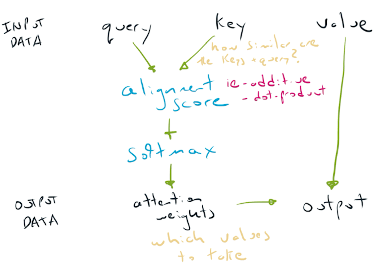
The three steps in an attention layer - alignment, softmax & key selection

Different attention layers (such as Additive Attention or Dot-Product Attention) use different mechanisms in the alignment step. The softmax & key selection steps are common to all attention layers.

Query, key and value

In the same way that understanding the time-step dimension is a key step in understanding recurrent neural networks, understanding what the query, key & value mean is foundational in attention.

A good analogy is with the Python dictionary. Let’s start with a simple example, where we:

• look up a query of dog
• to match with keys of dog or cat with values of 1 or 2 respectively
• and select the value of 2 based on this lookup of dog

query = 'dog'
#  keys = 'cat', 'dog', values = 1, 2
database = {'cat': 1, 'dog': 2}
database[query]
#  2

In the above example, we find an exact match for our query 'dog'. However, in a neural network, we are not working with strings - we are working with tensors. Our query, keys and values are all tensors:

query = [0, 0.9]
#  keys = [0, 0], [0, 1] values = [0], [1]
database = {[0, 0]: [0], [0, 1]: [1]}

Now we don’t have an exact match for our query - instead of using an exact match, we instead can calculate a similarity (i.e. an alignment) between our query and keys, and return the closest value:

database.similarity(query)
#  [1]

Small technicality - often the keys are set equal to the values. This simply means that the quantity we are doing the similarity comparison with is also the quantity we will place attention over.

Attention mechanisms

By now we know that an attention layer involves three steps:

1. alignment based on similarity,
2. softmax to create attention weights,
3. choosing values based on attention.

The second & third steps are common to all attention layers - the differences all occur in the first step - how the alignment on similarity is done.

We will briefly look at two popular mechanisms - Additive Attention and Dot-Product Attention. For a more detailed look at these mechanisms, have a look at the excellent Attention? Attention! by Lilian Wang.

Additive Attention

This first use of attention (known as Bahdanau or Additive Attention) addressed one of the limitations of the seq2seq model - namely the use of a fixed length context vector.

As explained in the LSTM section, the basic process in a seq2seq model is to encode the source sentence into a fixed length context vector. The issue is with all of the information from the encoder must pass through the fixed length context vector. Infomation from the entire source sequence is squeezed through this context vector inbetween the encoder & decoder.

In Bahdanau et. al 2015, Additive Attention is used to learn an alignment between all the encoder hidden states and the decoder hidden states. As the sequence is processed, the output of this alignment is used in the decoder to predict the next token.

Dot-Product Attention

A second type of attention is Dot-Product Attention - the alignment mechanism used in the Transformer. Instead of using addition, the Dot-Product Attention layer uses matrix multiplication to measure similarity between the query and the keys.

The dot-product acts like a similarity between the keys & values - below is a small program that plots both the dot-product and the cosine similarity for random data:

from collections import defaultdict

import matplotlib.pyplot as plt
import numpy as np
from scipy.spatial.distance import cosine

data = defaultdict(list)
for _ in range(100):
    a = np.random.normal(size=128)
    b = np.random.normal(size=128)
    data['cosine'].append(cosine(a, b))
    data['dot'].append(np.dot(a, b))

plt.figure(figsize=(10, 10))
_ = plt.scatter(data['cosine'], data['dot'])
plt.xlabel('cosine')
plt.ylabel('dot-product')

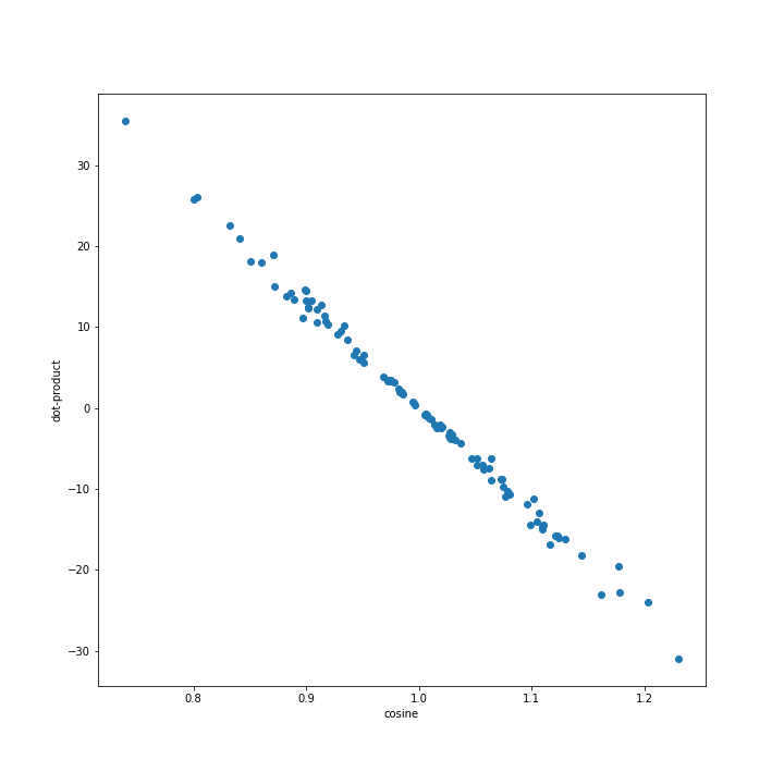
The relationship between the cosine similarity and the dot-product of random vectors

Implementing a Single Attention Head with the Keras Functional API

Dot-Product Attention is important as it forms part of the Transformer. As you can see in the figure below, the Transformer uses multiple heads of Scaled Dot-Product Attention.

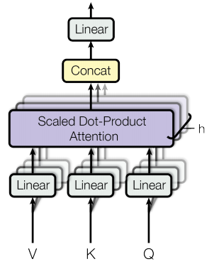
The multi-head attention layer used in the Transformer

The code below demonstrates the mechanics for a single head without scaling - see Transformer Model for Language Understanding for a full implementation of a multi-head attention layer & Transformer in Tensorflow 2.

import numpy as np
import tensorflow as tf
from tensorflow.keras import Input, Model
from tensorflow.keras.layers import Dense

qry = np.random.rand(4, 16, 32).reshape(4, -1, 32).astype('float32')
key = np.random.rand(4, 32).reshape(4, 1, 32).astype('float32')
values = np.random.rand(4, 32).reshape(4, 1, 32).astype('float32')

q_in = Input(shape=(None, 32))
k_in = Input(shape=(1, 32))
v_in = Input(shape=(1, 32))

capacity = 4
q = Dense(4, activation='linear')(q_in)
k = Dense(4, activation='linear')(k_in)
v = Dense(4, activation='linear')(v_in)

score = tf.matmul(q, k, transpose_b=True)
attention = tf.nn.softmax(score, axis=-1)
output = tf.matmul(attention, v)

mdl = Model(inputs=[q_in, k_in, v_in], outputs=[score, attention, output])
sc, attn, out = mdl([qry, key, values])
print(f'query shape {qry.shape}')
print(f'score shape {sc.shape}')
print(f'attention shape {attn.shape}')
print(f'output shape {out.shape}')
"""
query shape (4, 16, 32)
score shape (4, 16, 1)
attention shape (4, 16, 1)
output shape (4, 16, 4)
"""

This architecture also works with a different length query (now length 8 rather than 16):

qry = np.random.rand(4, 8, 32).reshape(4, -1, 32).astype('float32')
sc, attn, out = mdl([qry, key, values])
print(f'query shape {qry.shape}')
print(f'score shape {sc.shape}')
print(f'attention shape {attn.shape}')
print(f'output shape {out.shape}')
"""
query shape (4, 8, 32)
score shape (4, 8, 1)
attention shape (4, 8, 1)
output shape (4, 8, 4)
"""

What hyperparameters are important in an attention layer?

When using attention heads as shown above, hyperparameters to consider are:

• size of the linear layers used to transform the query, values & keys
• the type of attention mechanism (such as additive or dot-product)
• how to scale the alignment before the softmax (often done using the square-root of the length of the layer)

When should I use an attention layer?

Attention layers should be considered for any sequence problem. Unlike recurrent neural networks, they can be easily parallelized, making training fast. Fast training means either cheaper training, or more training for the same amount of compute.

The Transformer is a sequence model without recurrence (it doesn’t use an LSTM), allowing it to be trained without backpropagation through time.

One additional benefit of an attention layer is being able to use the alignment scores for interpretability - similar to how we can use the hidden state in an LSTM as a representation of the sequence.

Summary

I hope you enjoyed this post and found it useful! Below is a short table summarizing the article:

Layer	Intuition	Inductive Bias	When To Use
Fully connected	Allow all possible connections	None	Data without structure (tabular data)
2D convolution	Recognizing spatial patterns	Local, spatial patterns	Data with spatial structure (images)
LSTM	Database	Sequences & memory	Never - use Attention
Attention	Focus on similarities	Similarity & limit information flow	Data with sequential structure

---

Thanks for reading!

If you enjoyed this post, check out Artificial Intelligence, Machine Learning and Deep Learning.