Average vs. Marginal Carbon Intensities in Electricity Grids
Many energy professionals are (still!) getting this wrong.
Electricity carbon intensities are an essential part of the clean energy transition. Estimations & predictions of carbon intensities can drive decisions that clean up electricity grids.
Carbon intensities are challenging - there are different kinds of carbon intensity. This post will help to shine light on this important energy & climate topic.
In this post we will learn:
- what a carbon intensity is & how to calculate them,
- the two kinds of average carbon intensities,
- what average and marginal carbon intensities are,
- why the average carbon intensity is best for inventory, global carbon accounting,
- why the marginal carbon intensity is best for short term decisions,
- about a few problems with the marginal carbon intensity.
Context
A carbon intensity is the environmental equivalent of an electricity price - it is a signal that tells us something about the environmental health of the electricity grid.
There are multiple ways to estimate carbon intensity. Most common is the average carbon intensity - less common the marginal carbon intensity.
These two different quantities have different uses, and are not directly interchangeable. They should be looked at as any statistic - one estimate of a single quality of a distribution of numbers, applicable in some situations and not in others.
Interval level carbon intensity data is not often as available as electricity prices. Carbon intensities are often derived by joining together at least two datasets (commonly grid generation & generator carbon intensities). A more ambitious analysis would also consider how to handle the difference between generation & demand, or behind the meter generation - joining on even more data to do so.
Data focused clean tech companies like Tomorrow have made positive movements towards making carbon intensity data available - yet even they are still figuring out how best to use carbon intensities in electricity systems .
What is a carbon intensity?
A carbon intensity tC/MWh measures how carbon emissions tC change with electricity consumption MWh. A carbon intensity lets us calculate the amount of carbon in electricity, in the same way an electricity price $/MWh allows us to calculate the amount of money in electricity.
If we estimate an energy efficiency project will save 438 MWh of electricity - knowing the carbon intensity associated with this electricity was 0.1 tC/MWh means we can calculate a carbon saving of 43.8 tC - this is an example of the equation below:
carbon (tC) = carbon_intensity (tC/MWh) * electricity (MWh)
The valuable part of that equation in business contexts is often the tC - being able to estimate how much carbon we generate or save for some amount of electricity.
When doing the data work, often this equation is re-arranged. A similar calculation can be done from the electricity consumption of an entire grid - if we measure a grid consumption of 400 MWh and 200 tC, this implies a carbon intensity of 0.5 tC/MWh - an example of the equation below:
carbon_intensity (tC/MWh) = carbon (tC) / electricity (MWh)
A tale of two averages
Our first challenge with carbon intensities is the two different types of an average carbon intensity. This distinction is important when communicating with others - it’s possible you can be talking about different averages.
The first kind of average carbon intensity is an annual average carbon intensity. The second kind is an interval level average carbon intensity.
To demonstrate the difference we can run through an example. Let’s start with historical generation data - how much energy a generator produced in a given interval of time:
| Datetime | Solar MWh | Gas MWh | Electricity MWh |
|---|---|---|---|
| 2020-01-01T00:00:00 | 40 | 20 | 60 |
| 2020-01-01T00:30:00 | 60 | 10 | 70 |
In addition to this interval level data, we need to make assumptions about the carbon intensity of solar and gas. With real grid data these assumptions are often for individual generators.
For our example we will assume a carbon intensity of 0 tC/MWh for solar and 0.4 tC/MWh for gas. This then allows us to calculate an average carbon intensity for each interval:
| Datetime | Solar MWh | Gas MWh | Electricity MWh | Carbon tC | Carbon intensity tC/MWh |
|---|---|---|---|---|---|
| 2020-01-01T00:00:00 | 40 | 20 | 60 | 8 | 0.134 |
| 2020-01-01T00:30:00 | 60 | 10 | 70 | 4 | 0.057 |
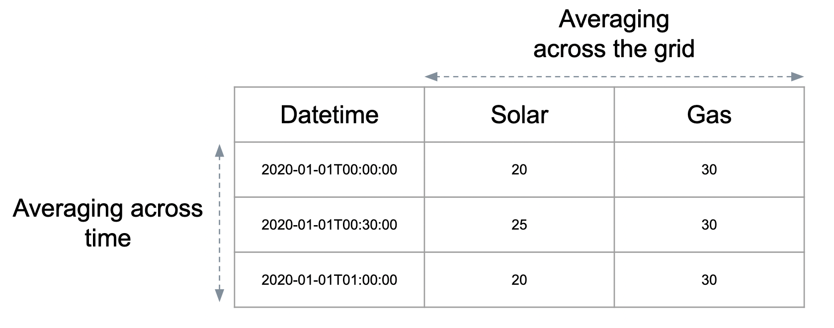
These two carbon intensities of 0.134 & 0.057 are interval level average carbon intensities. They average across the grid - not across intervals.
Using our friendly equation from before now calculate an annual average carbon intensity:
carbon_intensity (tC/MWh) = carbon (tC) / electricity (MWh) = (8 + 4) / (60 + 70) = 0.092
Note that we do not average averages here - calculating the annual average carbon intensity by taking the average of the two interval level intensities (0.134 + 0.057) / 2 = 0.096 - this would be incorrect. Using this average of averages would not allow us to recover tC from our average - we would incorrectly calculate 0.096 * (60 + 70) = 12.48 tC.
The average carbon intensity is useful for doing inventory accounting - understanding how much carbon is being emitted in total, and then apportioning all this carbon onto all the electricity demand. This can then be re-weighted by the fractions of that demand.
It’s useful when you want to equally smear carbon emissions over a large amount of electricity use - for example to understand how much of the total grid emissions a person or company is responsible for.
Note it’s also possible to have an annual average marginal carbon intensity as well - where we take the marginal generator across the grid and average across time.
The key takeaways here is that there are two opportunities to average a carbon intensity - once across the grid and once across time. Three of the most common combinations are below:
| Carbon Intensity | Grid aggregation | Time aggregation |
|---|---|---|
| Annual average | Average across all generators | Average across all times |
| Interval level average | Average across all generators | None |
| Interval level marginal | Select marginal generator | None |
Average & marginal train tickets
A central challenge with carbon intensities is understanding the difference between average and marginal. These are two different choices for how we aggregate across the grid - or more generally, across a market.
The difference can be demonstrated by comparing two markets - one for train tickets and one for electricity.
Two train tickets are purchased early for $20 each. A final ticket is purchased on the day, costing $100. These three tickets fufil our entire market demand for train tickets.
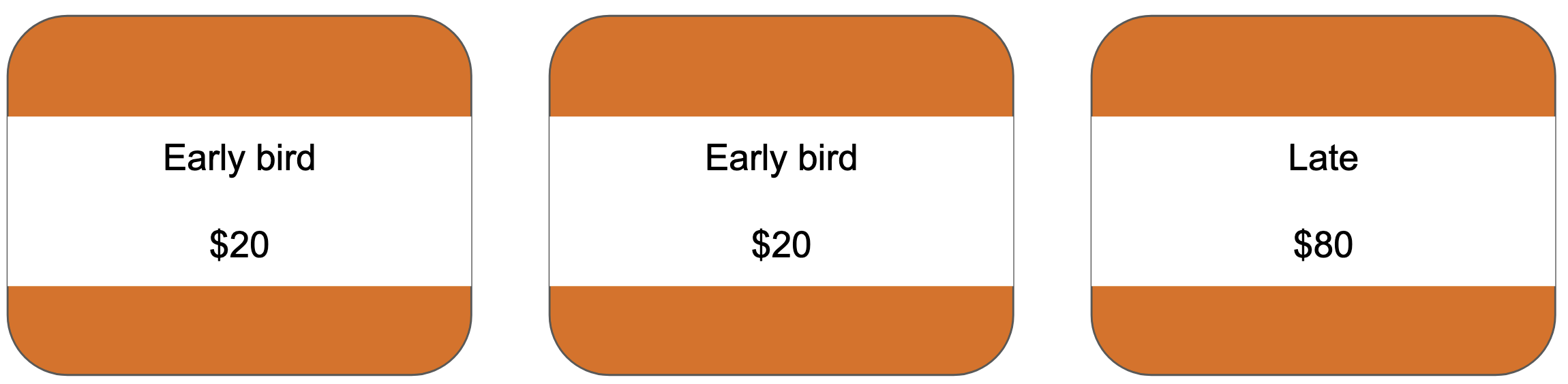
Let’s now ask a simple question - what is the price of a train ticket?
We can see there are three prices - one for each ticket purchaser. These three prices are marginal prices for each consumer. In the market for train tickets, everyone pays their marginal price.
These prices are the equivalent of a bid price or carbon intensity in an electricity grid. They can be stacked together into a bidstack - a view of the entire market.
For the train tickets, the average price is $46.67. This price is uninformative to the individual customer - no one actually paid $46.67 for a ticket! It would be informative to the user who wanted to compare how expensive this train market was versus another train market.
Let’s now compare this with an electricity market that settles based on marginal prices.
Three bids are accepted - all for 20 MWh of electricity. Two bids are at low prices, with a higher price bid being the final, marginal bid. These three bids fulfil our entire market demand of 60 MWh for electricity.
We can create a bid stacks for the two markets (train tickets & wholesale electricity market). The bid stack shows volume on the X axis and price on the Y axis - the bid stacks show all our bids for both markets:
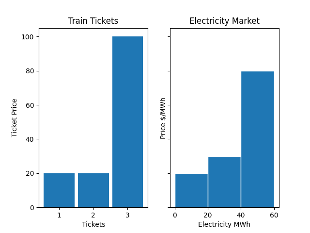
In markets like the National Electricity Market (NEM) in Australia, this final bid sets the price for the entire market. Every consumer of electricity will pay the marginal price of the most expensive generator. Quite different from our train tickets, where each customer pays their own marginal price.
These bid stacks alone don’t tell us everything about a market - notably in the case of the electricity grid where everyone pays a single settlement price - typically the marginal price of the most expensive generator (the price they bid & are dispatched at).
Let’s finally finish our medley of analogies by relating this back to average and marginal carbon intensities.
It’s not appropriate to create a bid stack of carbon intensities (maybe one day we run our electricity dispatch that way!). There is no market for the carbon intensity of electricity - our dispatch here has been done on price only.
We can however attach carbon intensities to each of our bids - representing how much carbon is associated with that bid’s volume of electricity.
| Bid Volume | Bid Price | Carbon Intensity |
|---|---|---|
| 20 | 20 | 0.1 |
| 20 | 30 | 0.1 |
| 20 | 80 | 0.6 |
Here we can calculate the average intensity as 0.27 tC/MWh.
The marginal carbon intensity here would be 0.6 tC/MWh - this is the carbon intensity of our most expensive market participant.
This is strong difference!
Marginal, counterfactual thinking
The marginal carbon intensity is relevant when we want to understand the short term impact of a decision on the electricity grid.
The marginal impact is the direct impact you had on the grid - the delta between the world where you acted and the world that you didn’t act.
If we are a battery that wants to discharge 5 MW at the most environmentally beneficial point will want to discharge when the marginal carbon is the highest.
In theory, this 5 MW will lead to a reduction in demand of 5 MW. This reduced demand means 5 MW less of generation needs to be secured in the wholesale market - and this 5 MW will come entirely off a single generator - the marginal generator.
The correct carbon intensity to consider when operating our battery is that of the marginal generator only - we do not care about what happened on the rest of the grid - only in the delta between the world where we did act and the world where we didn’t.
Problems at the margin
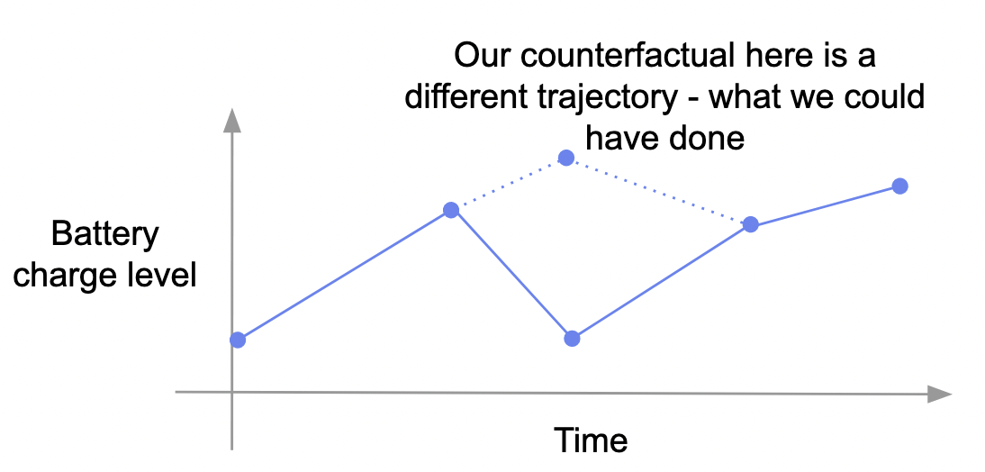
Thinking in terms of marginal carbon intensities means thinking about counterfactuals - what will be the net carbon effect of changing electricity consumption?
Understanding this counterfactual world requires understanding the mechanics & rules of how a grid responds to a change in electricity consumption. This makes marginal carbon intensities challenging.
This counterfactual problem also bites in other areas of energy - particularly in demand side flexibility, where the counterfactual is needed to establish the benefit of a demand side action.
Above we were looking at a wholesale electricity market - this made it possible for us to reason about the counterfactual world (it would reduce generation on the most expensive generator).
Two scenarios quickly harm our ability to reason even in this simple market. For very large changes in demand, the reduction in volume may spread multiple across multiple generators. Dispatch algorithms can often react in complex ways (with the dispatch changed both up and down on multiple participants) to a reduction in demand. Local network constraints can drive in deltas in dispatch that are hard to predict.
At the very small margin (~ 5 kW) - these fluctuations in demand are so small they will never actually lead to a different dispatch & change in load on the marginal generator.
These are likely just sucked up in frequency control - the collection of services grid operators use to balance the grid in real time (think seconds, not 30 minutes).
A final problem occurs with how bouncy a marginal carbon signal can be. It’s possible for the marginal generator to wildly vary from interval to interval - with the marginal generator in one interval having a much different carbon intensity than the interval before.
Another problem with the marginal carbon intensity is challenges of data availability, calculating the carbon intensities and the difficulty of predicting them for control.
The final problem with marginal approach, even if we could be accurate in terms of modelling how the grid responds, will never be able to target generation in the middle of the stack.
Often in the NEM the marginal generator can be hydro, with dirtier coal generation sitting lower in the bid stack.
If we imagine a grid with a baseload of renewables & coal, with balancing & marginal generator done in gas, then focusing on the marginal intensity only will only ever offset one type of generation - with no opportunities to reduce load on the coal generation.
This is a point directly made by Tomorrow - it’s a real flaw in focusing only on the margin that you miss out on targeting the rest of the stack.
Bringing more statistics to carbon intensities
These problems are not the end of the road - as an industry we must continue to work on figuring out how to model carbon intensities to clean up the grid - in both the short and long term.
One idea to target middle of the bid stack, dirty generation would be to aggregate by taking the dirtiest generator across the grid - this would incentivize dispatch to target these time periods to reduce demand far enough to start to displace that dirty generation.
Further reading:
- Marginal emissions: what they are, and when to use them,
- Marginal vs average: which one to use in practice?.
Thanks for reading!
If you enjoyed this, check out The Space Between Money and the Planet.