A simple Python workflow for time series simulations

A common workflow I encounter in my data science work is simulating a process through time. I often want to:

• simulate a process
• collect the results at each step
• output a simple plot of the variables over time

In this post I introduce a simple Python implementation for this that works really well.

For those in a rush I’ll first introduce the key components separately. I’ll then show how this simple framework is used to tackle a problem from the machine learning classic Sutton & Barto - An Introduction to Reinforcement Learning.

I’m in love with defaultdict, and I feel fine

The first component is a defaultdict from the collections module in the Python standard library. The advantage of a defaultdict is flexibility - instead of needing to initialize a key/value pair, you can add keys on the fly and append to an already initialized list.

#  if we use a normal python dictionary, adding a new key requires the following
stats = {}
stats['variable'] = []
stats['variable'].append(var)

#  adding another variable requires two more lines
stats['other_variable'] = []
stats['other_variable'].append(other_var)

#  if we instead use a defaultdict, we can do the five lines above in three lines
stats = defaultdict(list)
stats['variable'].append(var)
stats['other_variable'].append(other_var)

Having a dictionary full of lists is not particularly useful. But once our defaultdict is full of data, we can easily turn it into a pandas DataFrame using the from_dict method.

We need to make sure that all of the values in our stats dictionary are lists of the same length. This will be the case if we added one value for each variable at each step.

stats = pd.DataFrame().from_dict(stats)

Finally, we can use this dataframe with matplotlib to plot our data.

fig, axes = plt.subplots()
stats.plot(y='variable', ax=axes)
stats.plot(y='other_variable', ax=axes)

Example - updating the value function for a bandit

Now lets look at this framework in the context of a real problem. The problem is the solution to a question posed in Section 2.6 of Sutton & Barto - An Introduction to Reinforcement Learning. To fully understand the problem I suggest reading the chapter - you can find the 2nd Edition online for free here.

The problem involves the incremental updating the value function for a bandit problem.

\[Q_{n+1} = Q_{n} + \alpha [R_{n} - Q_{n} ]\]

Sutton suggest that an improvement to using a constant step size (say \(\alpha=0.5\)) to use a step size \(\beta\).

\[\beta_{n} = \frac{\alpha}{\overline{o}_{n}}\]

Where we update \(\overline{o}_{n}\) by

\[\overline{o}_{n} = \overline{o}_{n-1} + \alpha (1-\overline{o}_{n-1})\]

The program written for this problem is given below. To get the figure to show, you need to first save the code snippet to bandit.py, then run the program in interactive mode ($ python -i bandit.py).

from collections import defaultdict

import matplotlib.pyplot as plt
import numpy as np
import pandas as pd


alpha = 0.0001
q = 10
omega = 0

stats = defaultdict(list)

for step in range(50):
    stats['q'].append(q)
    stats['omega'].append(omega)

    omega = omega + alpha * (1 - omega)
    beta = alpha / omega
    stats['beta'].append(beta)

    reward = np.random.normal(loc=5, scale=1)
    stats['reward'].append(reward)

    q += beta * (reward - q)

result = pd.DataFrame().from_dict(stats)

f, a = plt.subplots(nrows=4)

result.plot(y='reward', ax=a[0])
result.plot(y='q', ax=a[1])
result.plot(y='omega', ax=a[2])
result.plot(y='beta', ax=a[3])

print('final estimate {}'.format(stats['q'][-1]))

f.show()

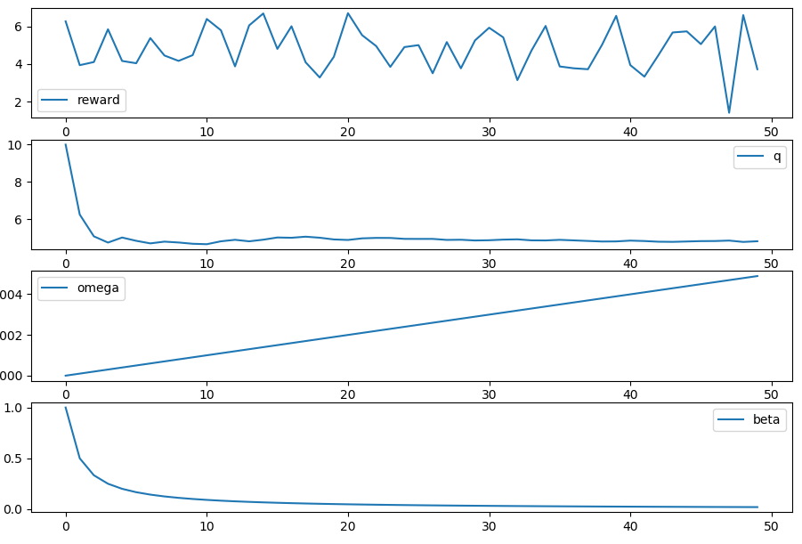
The results of the run are stored in the result DataFrame:

>>> result.head()
           q   omega      beta    reward
0  10.000000  0.0000  1.000000  4.762884
1   4.762884  0.0001  0.500025  4.623668
2   4.693273  0.0002  0.333367  4.734825
3   4.707125  0.0003  0.250038  4.573823
4   4.673794  0.0004  0.200040  3.663734

What pops out the end is a simple time series plot of how our variables changed over time:

Thanks for reading!