This is the final post in a three part series of debugging and tuning the energypy implementation of DQN. In the previous posts I debugged and tuned the agent using a problem - hypothesis - solution structure. In this post I share some final hyperparameters that solved the Cartpole environment - but more importantly ended up with stable policies.
The main changes that (I think!) contributed towards the high quality and stable policy were:
I ran four runs - two with an epsilon-greedy policy and two with a softmax policy. The experiments were run on the master branch of energypy at this commit.
The performance of the four agents is shown below in Figure 1. This environment (Cartpole-v0) is considered solved when the agent achieves a score of 195 over 100 consecutive episodes - which occurred after around 150,000 steps for the epsilon-greedy agents.
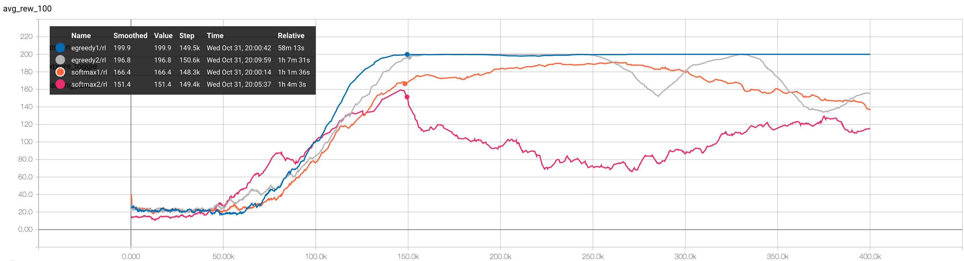
The epsilon-greedy policy outperformed the softmax policy - although I wasn’t quite sure how to decay the softmax temperature (in the runs above I decayed it from 0.5 to 0.1 over the experiment). The softmax policy implementation is shown below - it lives in the energypy library at energypy/common/policies/softmax.py.
softmax = tf.nn.softmax(tf.divide(q_values, temp), axis=1)
log_probs = tf.log(softmax)

entropy = -tf.reduce_sum(softmax * log_probs, 1, name="softmax_entropy")

samples = tf.multinomial(log_probs, num_samples=1)
policy = tf.gather(discrete_actions, samples)Previously I had been using much larger neural networks - typically three layers with 50 to 250 nodes per layer. For the Cartpole problem this is far too much! A smaller and shallower network has enough capacity to represent the action-value function for a high quality policy.
There is an argument for larger networks:
But on the other hand:
Increasing the number of steps between target network updates and lowering the learning rate both reduce the speed of learning but should give more stability. In reinforcement learning stability is the killer - although sample efficiency is a big problem in modern reinforcement learning you would rather have a slow, stable policy than a fast unstable one!
The idea behind increasing the size of the replay memory was to smooth out the distribution of the batches. What I was quite often seeing was good performance up to the first 100,000 steps followed by collapse - so I thought that maybe the agent was suffering with changes in distribution over batches as it learnt. Cartpole doesn’t have a particularly complex state space, so it’s likely that all states are useful for learning throughout an agent’s lifetime.
The hyperparameters used in the four Cartpole runs are shown below:
[DEFAULT]
total_steps=400000
agent_id=dqn
policy=e-greedy
discount=0.9
update_target_net=10000
tau=1.0
batch_size=512
layers=8, 4
learning_rate=0.0001
learning_rate_decay=1.0
epsilon_decay_fraction=0.4
initial_epsilon=1.0
final_epsilon=0.01
memory_fraction=1.0
memory_type=array
double_q=True

[softmax1]
policy=softmax
epsilon_decay_fraction=1.0
initial_epsilon=0.5
final_epsilon=0.1
seed=5

[softmax2]
policy=softmax
epsilon_decay_fraction=1.0
initial_epsilon=0.5
final_epsilon=0.1
seed=42

[egreedy1]
policy=e_greedy
seed=5

[egreedy2]
policy=e_greedy
seed=42Because I’ve spent so much time tuning this DQN agent to Cartpole, I wanted to see if I was overfitting by looking at how the agent performed on another benchmark problem from gym, the Pendulum environment. This environment doesn’t have solved criteria - however the maximum possible reward per episode is 0. Figure 2 shows the performance of the same set of agents on Pendulum.
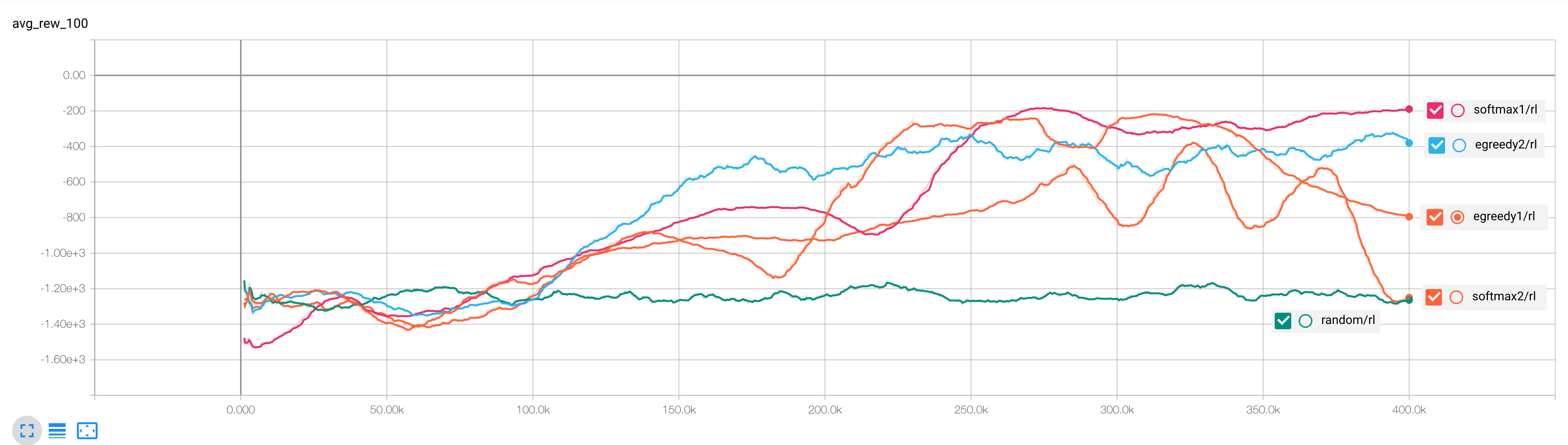
Pendulum has a continuous action space - I chose to discretize the space with five actions. It’s possible that this is too coarse of a discretization for the agent to find the optimal policy. It’s also possible that Pendulum might need a larger network to model the action-value function.
Stability, not speed, is the goal in reinforcement learning:
Thanks for reading!