This post continues the emotional hyperparameter tuning journey of implementing DQN for the CartPole environment.
This is part of a three-part series:
The code used to run the experiment is on this commit of energypy.
These posts follow a problem-hypothesis structure. Often the speed between seeing cause and effect is quick in computer programming. This allows a rapid cycling through hypotheses. In reinforcement learning, the long training time (aka the sample inefficiency) increases the value of taking the time to think about the problem relative to the cost of testing a hypothesis.
Interactive tuning has two benefits:
For all experiments I perform three runs over three different random seeds. These random seeds are kept constant for each experiment. The random seed for the environment action sampling is not kept constant - it is intentionally kept separate. A good discussion on why the Open AI library does this is here. This means that some randomness will be kept the same (i.e. neural network weight initialization), other sources of randomness won’t be.
Picking up where we left off in the first post - the major problem was instability. The agent was often able to solve the CartPole-v0 environment (Open AI consider this environment solved when an average over the last 100 episodes of 195 is reached). But after solving the environment the agents often completely forgot what they had learnt and collapsed to poor policies.
My hypotheses for the cause of the policy quality collapse were:
I then progressed to semi-scientifically investigate these hypotheses.
The hypothesis at this stage was that overestimation bias was causing instability - I also wanted to try out the DDQN code.
Overestimation bias is the tendency of Q-Learning algorithms to overestimate the value of states. This overestimation is a result of the aggressive acting and learning in the Q-Learning algorithm:
Double Q-Learning (and it’s deep learning variant DDQN) aims to overcomes this overestimation bias by selecting actions according to the online network, but quantifying the return for this action using the target network.
Because DQN already has the target network, modifying it to DDQN requires only a few changes - one of which is below. An argmax is performed over the online network evaluation of the value of the next state. The index of this argmax is then used with the target network values of the next state.
if self.double_q:
online_actions = tf.argmax(self.online_next_obs_q, axis=1)
unmasked_next_state_max_q = tf.reduce_sum(
self.target_q_values * tf.one_hot(online_actions, self.num_actions),
axis=1,
keepdims=True,
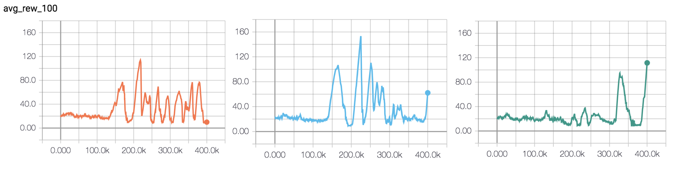
)The main hyperparameters for the first experiment looking at the effect of DDQN were:
total_steps = 400000
discount = 0.99
tau = 0.001
learning_rate = 0.0005
learning_rate_decay = 0.1
epsilon_decay_fraction - 0.05
memory_fraction = 0.2
double_q = True
gradient_norm_clip = 1.0
batch_size = 32
layers = 5, 5, 5
The results across three random seeds are shown in Figure 1.
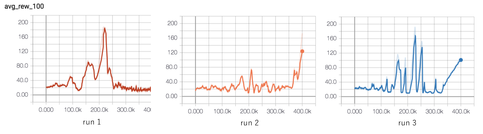
Figure 1 shows that the instability problem still exists! On to the next hypothesis.
In DQN the online network is changed at each step by minimizing the difference between the Bellman target and the current network approximation of Q(s,a). The hypothesis was that if the batch is too small (previously I was using batch_size=32) then the distribution of the data per batch won’t be smooth. These unsmooth updates hurt the policy stability.
In the CartPole environment, as the agent learns the episode length increases. As the episode length increases, the relative amount of terminal states in each batch will decrease. Knowing that the maximum episode length is 200 I increased the batch size to 256. Larger batch sizes allow higher learning rates, because the smoother distribution allows a higher quality gradient update.
Batch size is second only to learning rate in importance. Neural networks are trained using batches for multiple reasons:
In the 2015 DeepMind work, they used batch_size=32. Each state and next state was four images, so a single batch had 128 images. CartPole uses a small numpy array (and we train on CPU). So this potential constraint on batch size doesn’t apply.
For these simple reinforcement learning problems the idea is that smaller neural networks should be preferred, as they have less change to overfit.
One reason why a small neural network could cause instability is aliasing (sharing of weights). Aliasing could mean that changes to one part of the network disrupt the understanding encoded in another part of the network.
Up until now I have been using a neural network structure of 5, 5, 5 (i.e. 3 layers with 5 nodes per layer). My hypothesis was that even though this is not a lot of nodes, because the network has three layers there will be aliasing (i.e. changes in the input layer affect all the layers below it).
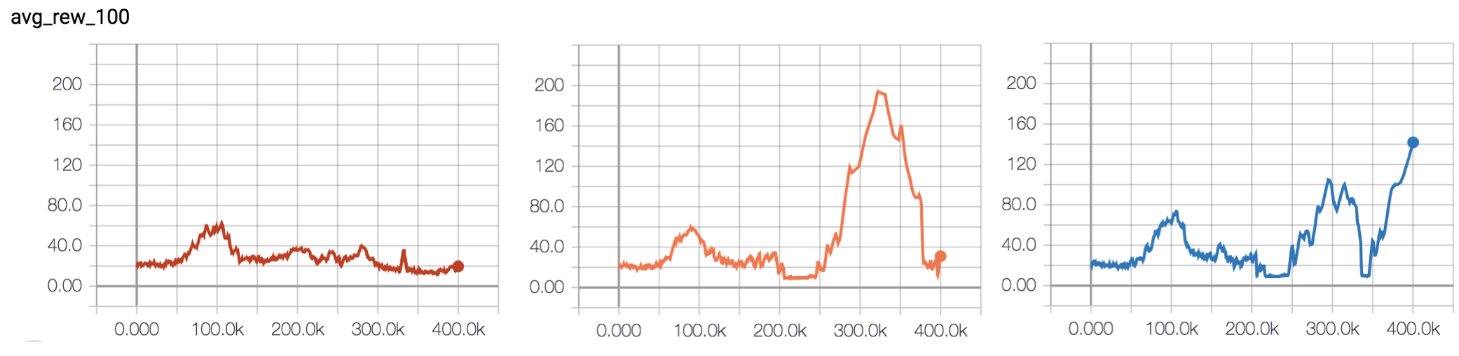
Updated hyperparameters were:
layers = 256, 256
batch_size = 256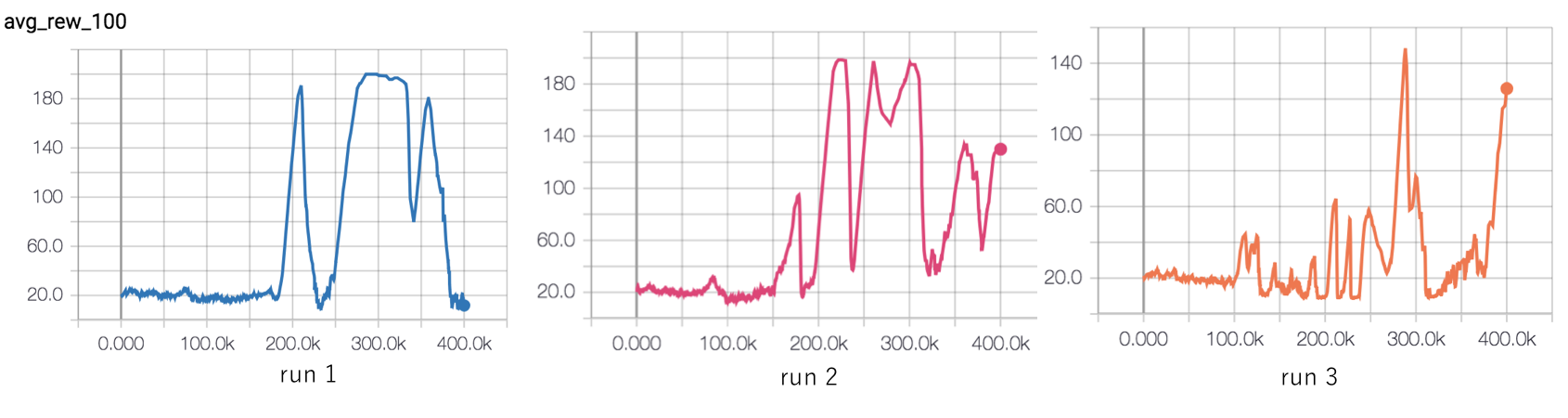
The batch size and neural network size changes do seem to have improved stability - the agents are able to stay at the maximum reward of 200 for a longer. The issue is that later in the experiment, the agents forget everything they have learnt and collapse to poor quality policies. Run 1 is especially disappointing!
The target network update is an obvious place where instability could arise. There are two common strategies for updating the target network:
C steps (C = 10k-100k steps in the 2015 DeepMind DQN work)I’ve been using the second strategy so far, with tau=0.001.
copy_ops = []
for p, c in zip(parent, child):
    assert p.name.split("/")[1:] == c.name.split("/")[1:]

    copy_ops.append(c.assign(tf.add(tf.multiply(p, tau), tf.multiply(c, 1 - tau))))
One issue with the tau=0.001 strategy is that perhaps a neural network has to be taken as a whole. Because of the massive connectivity, changing the value of one weight might lead to drastic changes in other parts of the network (a machine learning version of the butterfly effect). While the tau=0.001 strategy should allow a smoother and more gradual update, in fact it might cause instability.
Luckily the new energy-py implementation of DQN can easily handle both, by setting two parameters in the DQN agent __init__:
#  parameters to fully copy weights every 5000 steps
tau = 1.0
update_target_net = 5000

#  parameters to update a little bit each step
#  this is the strategy I had been using so far
tau = 0.001
update_target_net = 1
The hyperparameters for the different target net update experiment are below. I reduced the size of the neural network - the previous structure of 256, 256 seemed overkill for a network with an input shape of (4,) and output shape of (2,)!
batch_size = 256
layers = 128, 128
tau = 1.0
update_target_net = 5000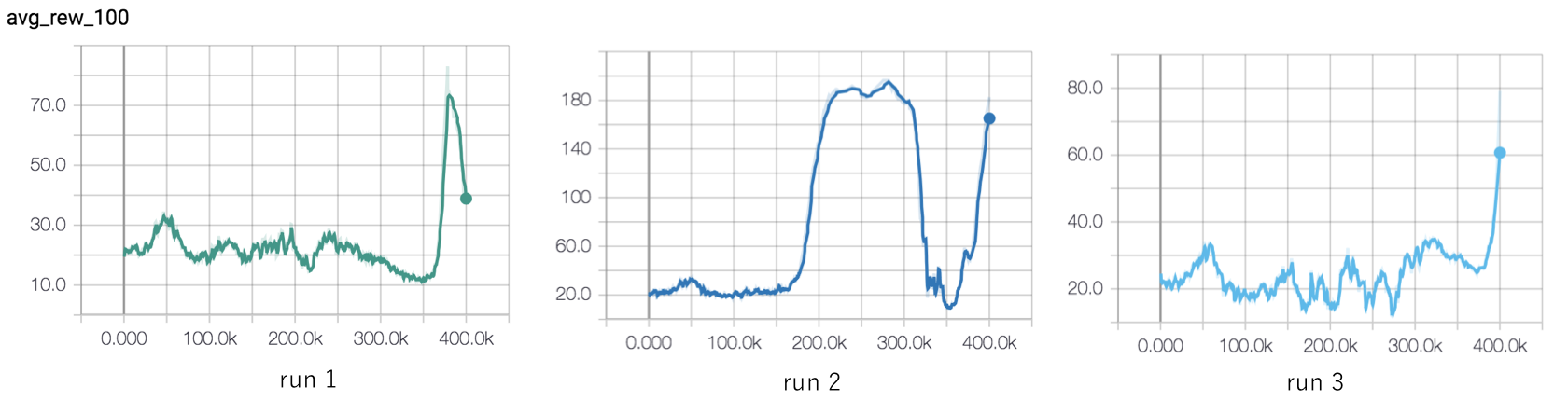
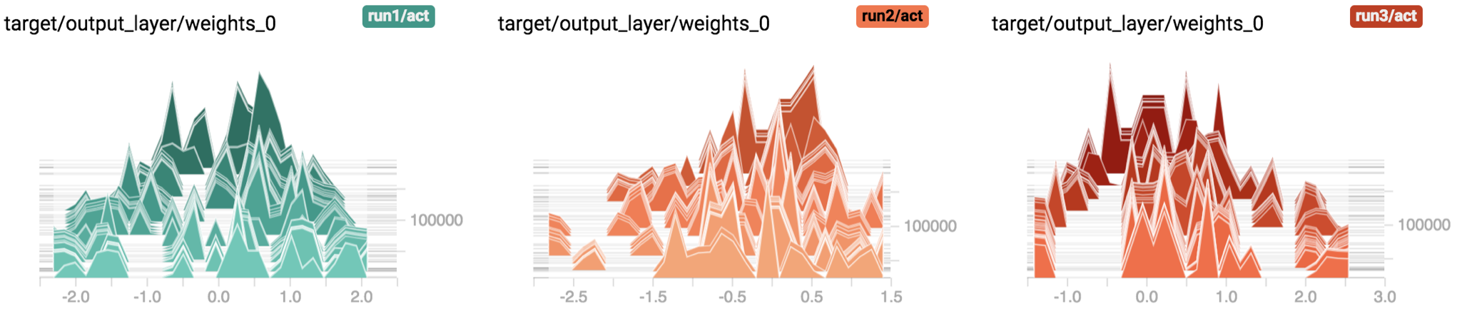
Figure 3 shows the target net update strategy slows learning. This is expected - rather than taking advantage of online network weight updates as they happen, the agent must wait until the target network reflects the agent’s new understanding of the world. Run 2 is especially promising, with the agent able to perform well for around 100k steps.
The main hyperparameter with this style of target network updating is the number of steps between updates. I ran a set of experiments with a quicker update (update_target_net=2500) to see if I could get learning to happen quicker and maintain of stability. The results for these runs are shown in Figure 4.
Looks like that didn’t work! By this point I started to get concerned that I was torturing hyperparameters too much (leading to a form of selection bias where I ‘overfit’ the implementation of DQN to this specific environment). So rather than continuing my (somewhat) scientific approach of changing only one thing at a time, I decided to try to combine all the lessons I had learnt and train the best agent I could. I gave myself two more experiments until I would force myself to stop.
Given that reducing the steps between target network updates seems to reduce performance, I decided to set update_target_net=10000. I also increased the learning rate and decreased the size of the neural network. Both of these changes were in the context of looking at lot of other implementations of DQN for the Cartpole environment.
I increased the learning rate to 0.001 to take advantage of the large batch size (256). A larger batch size should allow higher learning rates, as the gradient updates are higher quality. I reduced the size of the neural network to 64, 32 based on the feedforward structures I saw in other implementations.
While preprocessing Bellman targets is often given as advice for reinforcement learning, many DQN implementations (including the DeepMind 2015 implementation) don’t do any processing of the Bellman target. For this reason I decided to play around with the batch norm layer.
Up until now I was using tf.layers.batch_normalization with the Bellman target as follows:
self.bellman = self.reward + self.discount * self.next_state_max_q

bellman_norm = tf.layers.batch_normalization(
    tf.reshape(self.bellman, (-1, 1)),
    center=False,
    training=True,
    trainable=False,
)

error = tf.losses.huber_loss(
    tf.reshape(bellman_norm, (-1,)), self.q_selected_actions, scope="huber_loss"
)
I changed the batch norm arguments to default (i.e. training=False). In the tf.layers implementation of batch norm the layer will use historical statistics to normalize the batch. The effect of this on the Bellman target is quite dramatic.
bellman_norm = tf.layers.batch_normalization(
    tf.reshape(self.bellman, (-1, 1)),
    center=True,
    training=False,
    trainable=True,
)
Figure 6 shows the batch normed Bellman target with training=True (i.e. normalize each batch using the batch statistics) for the runs show in Figure 5 above. Figure 7 shows the Bellman target with training=False.
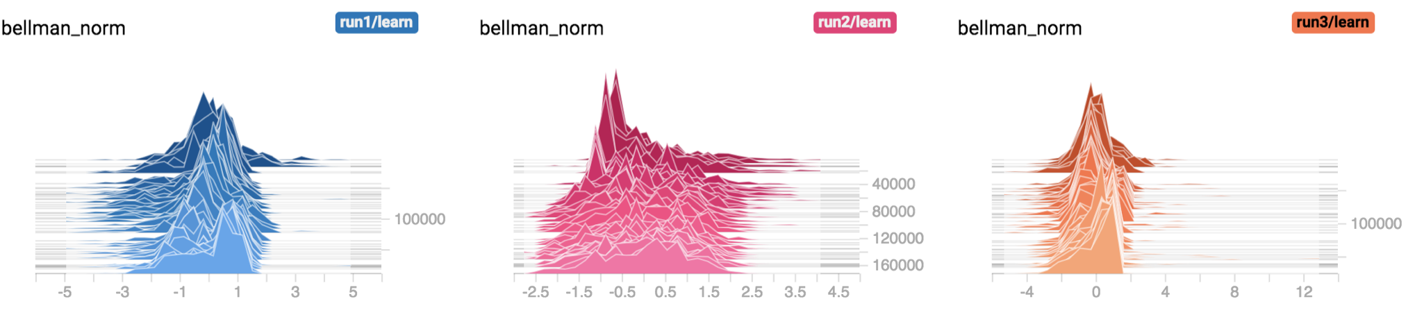
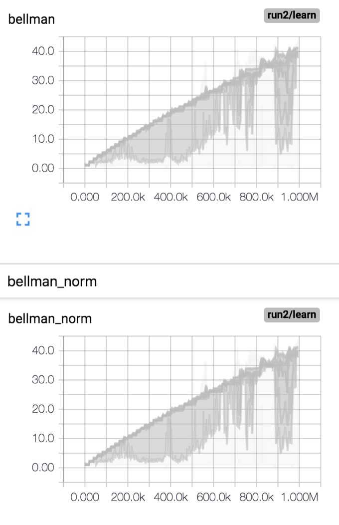
So it seems that using the batch norm layer with default parameters is essentially like not using it at all.
For the final run I increased the number of steps from 400k to 1000k. While this is a massive number of steps, the reality of reinforcement learning is that it is sample inefficient. While it’s possible that torturing hyperparameters can help with the sample inefficiency, another valid fix for sample inefficiency is more samples. This is equivalent to getting more data in a supervised learning setting.
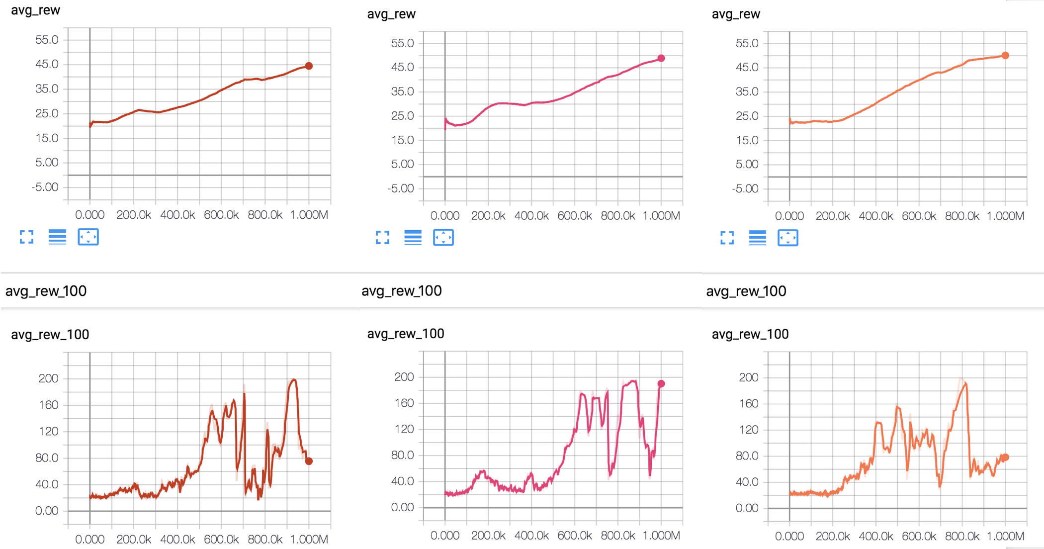
So after a whole heap of CPU time - what can we say about the final performance? All three runs do solve the environment (this environment is considered solved when an average of 195 is achieved over the last 100 episodes).
All three runs also show catastrophic forgetting - i.e. after they solve the environment they all managed to forget their good work. What then is the solution to this?
In supervised learning it is common to keep track of the validation loss (i.e. the loss on a test set) during training. Once this validation loss starts to increase, training is stopped (known as early stopping).
This is a potential solution to the stability problem. Rather than training forever, once good performance has been achieved training should stop.
If you think about how we learn skills in the real world, we do often use early stopping. Once we learn handwriting write to a decent level we commonly don’t continue to train the skill. Instead we fall into a repeated pattern of writing in the same way for the rest of our lives.
It’s perhaps cruel to continue to force gradient updates on an agent when it has solved an environment. A small enough learning rate should solve this problem but it’s likely that the learning rate would be so small that there is no point doing the update in the first place.
This process of debugging has been an emotional journey. It’s something I’m very glad I did - Yoshua Bengio often talks about how it’s crucial to ones development as a machine learning professional to spend the time training and debugging algorithms.
Key lessons learned:
While you can learn from reading, there is no replacement for getting your hands dirty. Spending the time training a whole bunch of models and hypothesizing what the effects of hyperparameters might be is time well spent.
When I was reviewing other implementations of DQN around GitHub or on blogs, I often saw a successful iteration in the blog post then a number of comments saying that the implementation didn’t work.
Thanks for reading!